Lecture Notes in Pattern Recognition: Episode 36 – Performance Measures on Finite Data

These are the lecture notes for FAU’s YouTube Lecture “Pattern Recognition“. This is a full transcript of the lecture video & matching slides. We hope, you enjoy this as much as the videos. Of course, this transcript was created with deep learning techniques largely automatically and only minor manual modifications were performed. Try it yourself! If you spot mistakes, please let us know!
Welcome back to Pattern Recognition! Today we want to look a bit more into model assessment. And then particularly, we want to know how to estimate the statistics and in particular the performance robustly on datasets of fixed size.
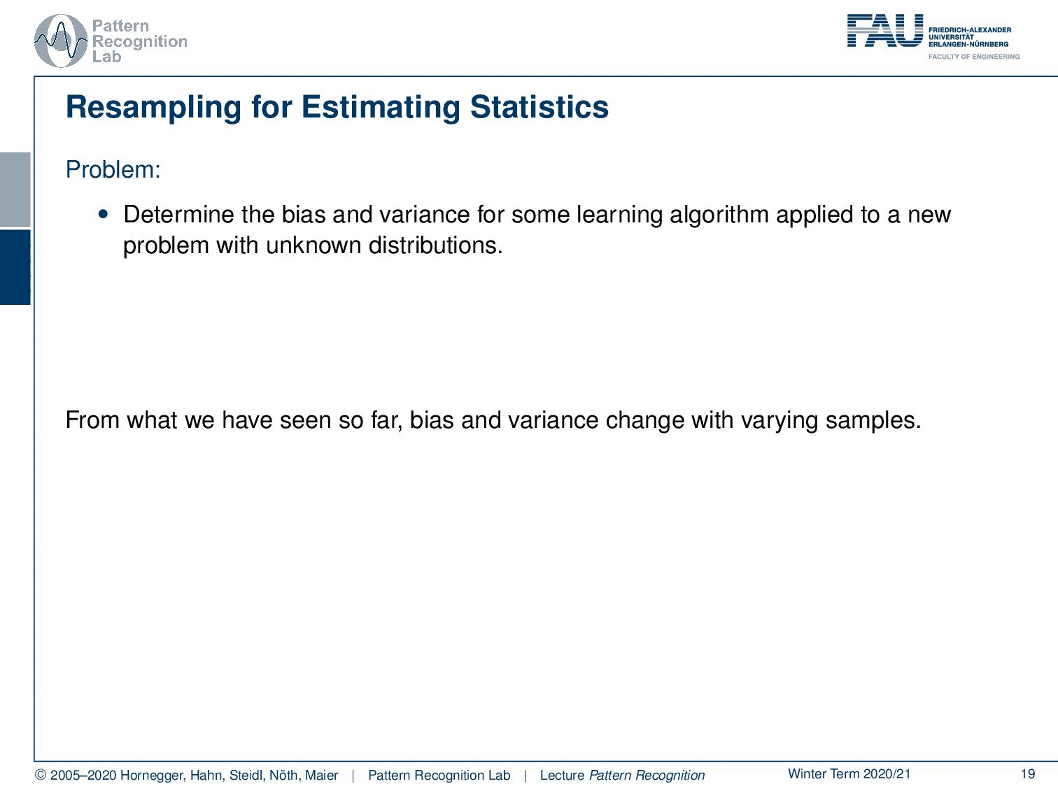
The problem is that you want to determine the bias and variance for some learning algorithm. And of course, we want to estimate this performance on data that we have not seen yet. So we want to estimate the performance for unknown distributions. From what we’ve seen so far, bias and variance change with varying samples. So we will need resampling techniques that can be used to create a more informative estimate of general statistics.
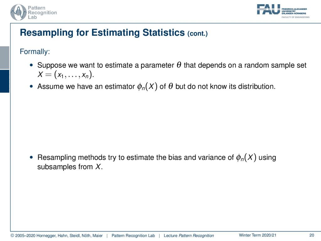
Formally, we can express this in the following way. Let’s suppose we want to estimate a parameter vector θ that depends on a random sample set that is given as X, ranging from x1 to xn. Then we can assume that we have an estimator of θ, but we do not know its distribution. So the resampling methods try to estimate the bias and variance of this estimator using the subsamples from X.
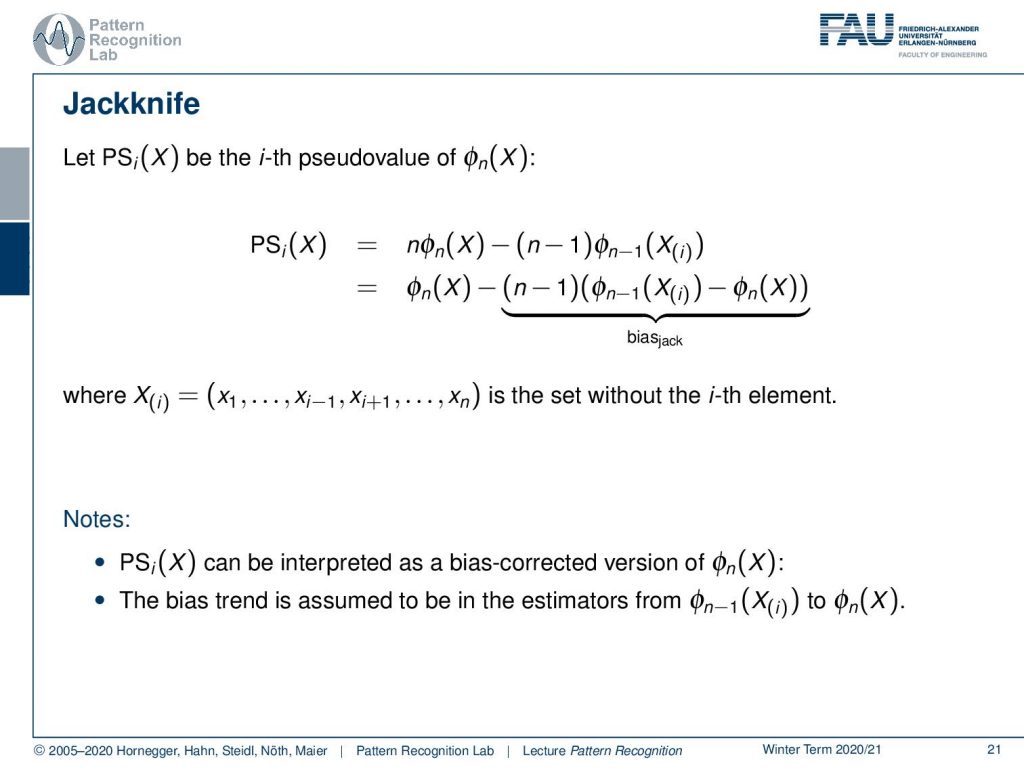
This brings us to the Jackknife. And the Jackknife is using the so-called pseudo value that we index here with i of x. This pseudo value is determined from the estimator in the following way: so you take n times the estimated value that is produced on X and then you subtract n-1 times the estimated value of the set where you’re omitting the element i. Then you can rewrite this, breaking essentially up the multiplication with n, and you pull the remaining estimate of X into the right-hand part. This then gives you n-1 and then the difference between the estimator where the element i is missing times the complete estimator. So you can essentially use this pseudo value to determine the performance of our estimator if the ith value is missing. You essentially estimate the bias between those two models and then you subtract it from the model that you estimated on the complete data. We assumed that the bias trend can be estimated from the difference between different estimations from different sets. And here we construct this by the difference between the estimators when we essentially omit one of the samples in the estimation process.
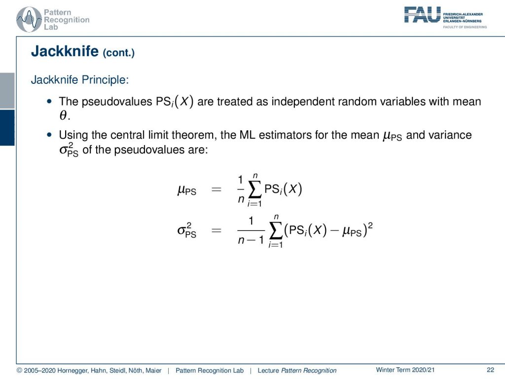
So essentially, the Jackknife principle is that the pseudo values are treated as independent random variables with mean θ. And then, using the central limit theorem, the maximum likelihood estimators for the mean and the variance of the pseudo values can be essentially determined as the mean over all the pseudo values. The variance is determined as 1 over n-1 and the sum over the differences of the pseudo values with the respective mean.
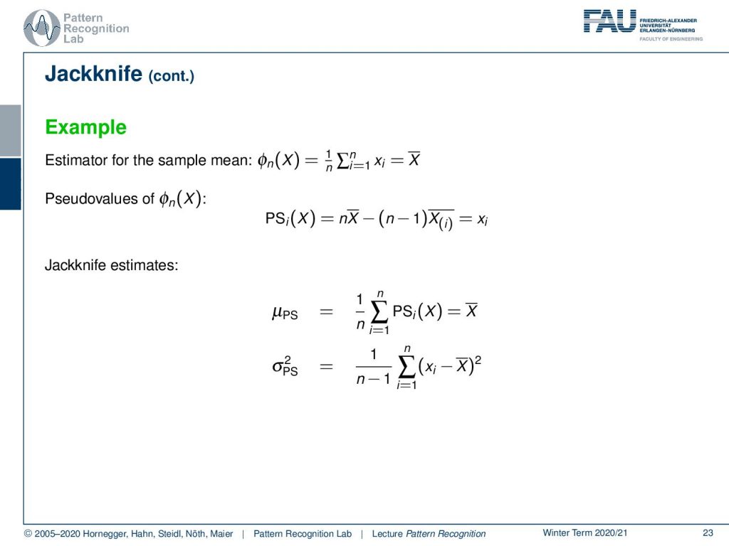
Let’s look into one example. Here, the estimator for the sample mean is given simply as the mean value of X. Now the pseudo values can be determined as n times the mean value of X minus (n-1) times the mean value where Xi is missing. If you write this up this is nothing else than xi. So you can then essentially determine the Jackknife estimate. And the Jackknife estimate is then simply given as the mean. So, here the mean doesn’t change in the Jackknifing, but you’ll see that the variance is changed. The variant is not normalized with one over n but with one over n minus one. So we tend to estimate a higher variance. You’ll see that if you have large sample numbers it doesn’t change that much, but if you have rather low sample numbers, then you generally have to estimate the variance higher than what you get from the typical ML estimate.
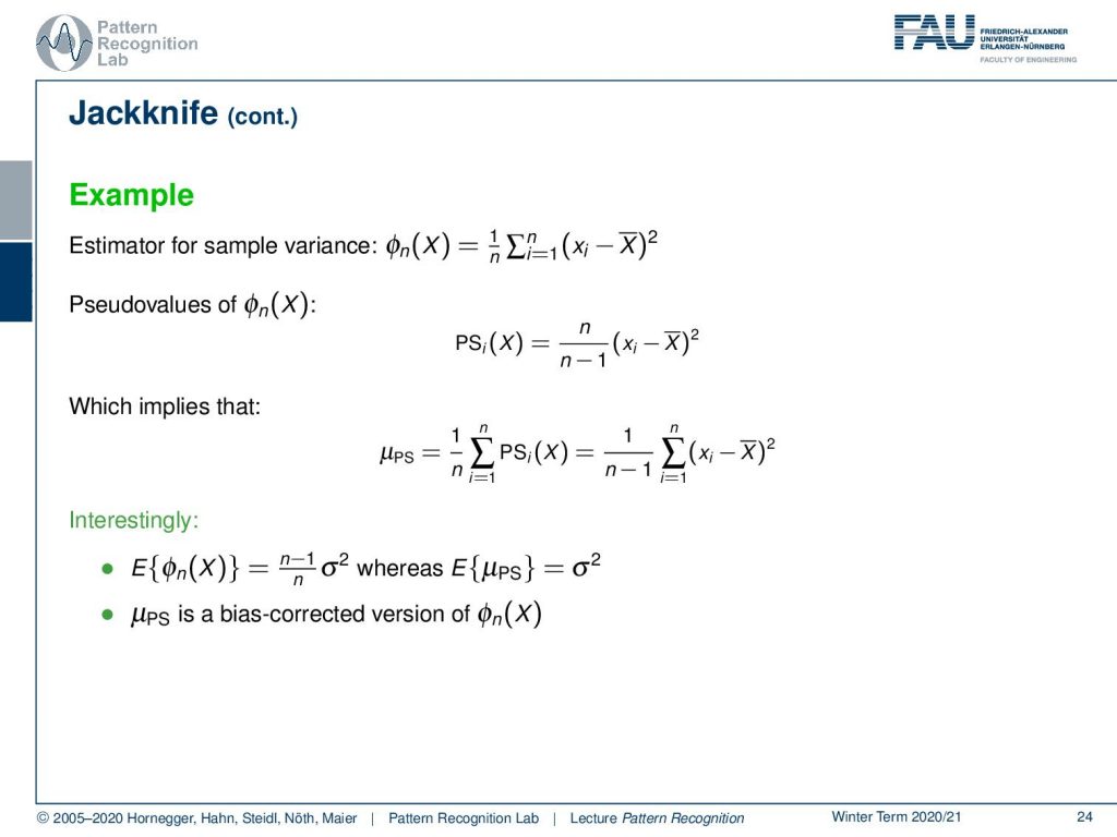
Let’s have a look into the case where the simple estimator is the variance. Here we take the mean value minus the samples and sum up, and this goes then up to one. Now we can again compute the pseudo values. And the pseudo values will then result in n over n minus one of xi minus the mean value of x. This way you can see that the mean of the Jackknife estimate is then found as the mean of the pseudo values. And this gives one over n minus one and the traditional variants estimate. So this is essentially the same result that we’ve seen on the previous slide. Now, this is quite an interesting observation. If you would compute the expected value for our estimator here in this case then you would get n minus one over n times the variance. And here in our Jackknife estimate, we get exactly the variance. so we could say the Jackknife estimate is a bias-corrected version of our estimator.
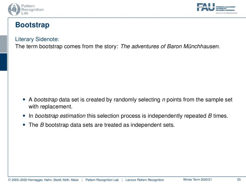
Let’s have a look at the bootstrapping procedure. I have a side note here that bootstrapping comes actually from the story “the adventures of Baron Münchausen” where he is trying to pull himself out of the mud just pulling on his own bootstraps. Bootstrapping is an idea where you create sub data sets by randomly selecting endpoints from the sample set with replacement. So in the bootstrap estimation, the selection process is independently repeated B times. This then leads to B bootstrap data sets that are treated as independent sets.
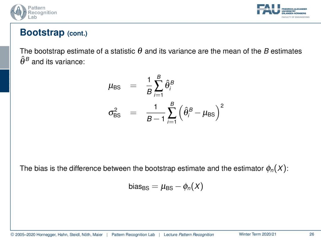
Then we can also do a bootstrap estimate of the statistic of θ and its variance based on the B mean estimates and its variance. And here you then can simply see that I estimate B̂ on the respective bootstrap subset and then we just average. And of course, we can also compute the variance for the same statistic. The bias is in the difference between the bootstrap estimate and the estimator. So this is then essentially giving us the bias.
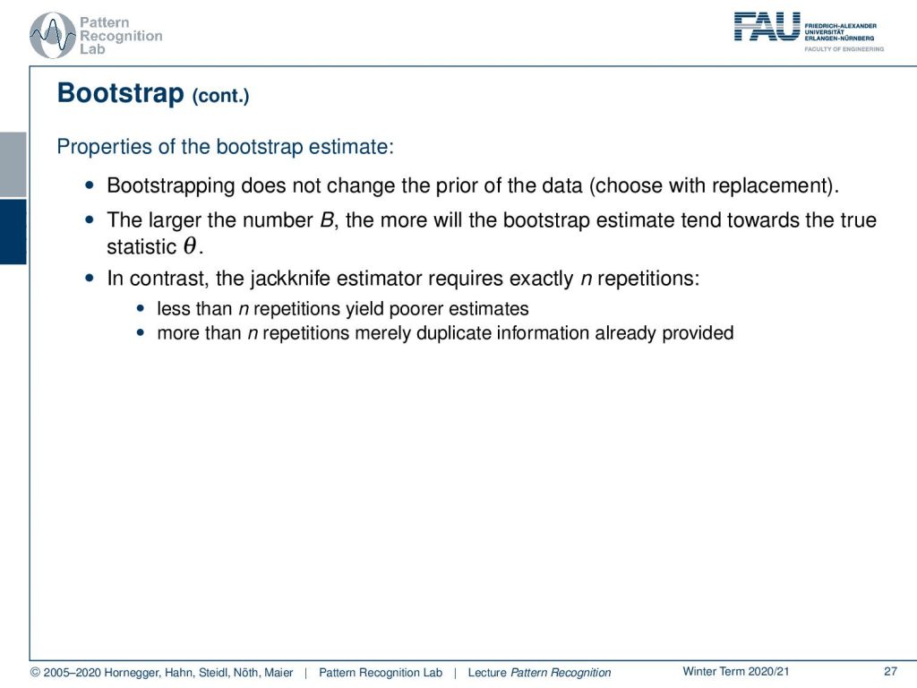
Now the properties of this bootstrap estimate are that bootstrapping does not change the price of the data because you choose with replacement. The larger the number B, the more the bootstrap estimate will tend towards the true statistic of θ. So in contrast to the Jackknife estimator, which requires exactly n repetitions so we can vary the number n here. If we have less than n repetitions, we probably have poorer estimates. And if I have more than n repetitions, we merely duplicate information that was already provided.
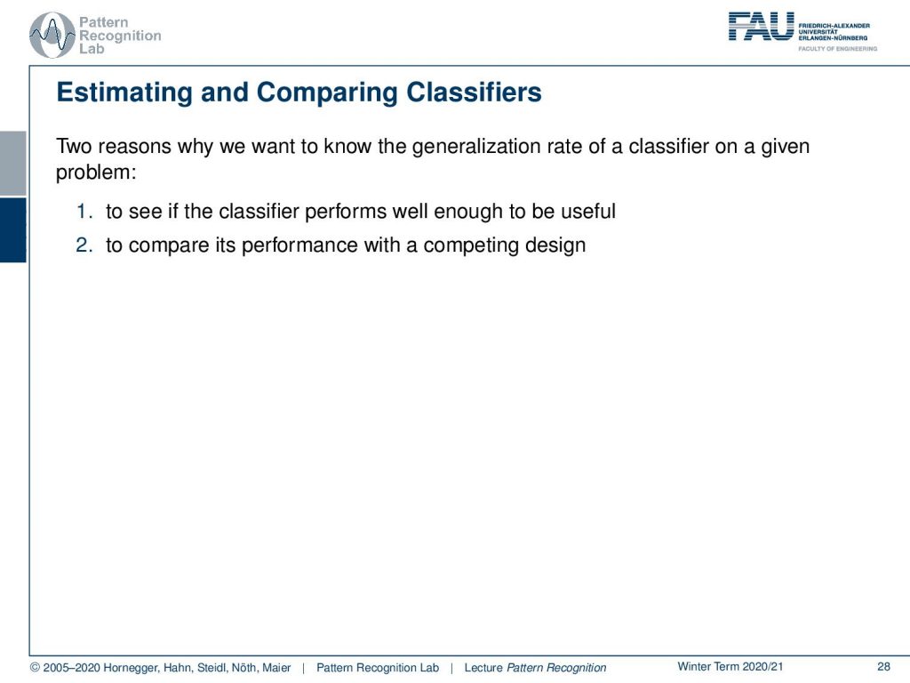
Let’s estimate and compare classifiers. There are, of course, several reasons why we want to know the generalization rate of a classifier on a given problem. We want to see if the classifier performs well enough to be useful, and we want to compare its performance with a competing design.
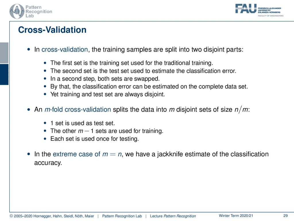
This then leads to the concept of cross-validation. Now cross-validation takes the training samples and splits them into disjoint parts. So you can use for example the first set for training. Then you traditionally train. Then the second set is used for testing to estimate the classification error. In a second step, you can just swap the two sets and by this, the classification error can be estimated on the complete dataset. Yet training and test are always disjoint. An m-fold cross-validation splits the data into m disjoint sets of size n over m. Then you use one set as a test set and the other m – 1 sets are used for training. And then you repeat this procedure m times such that each set is used once for training. In the extreme case of m = n, we have a Jackknife estimate of the classification accuracy. This is then also known as the leave one sample out or leave one out estimation procedure.
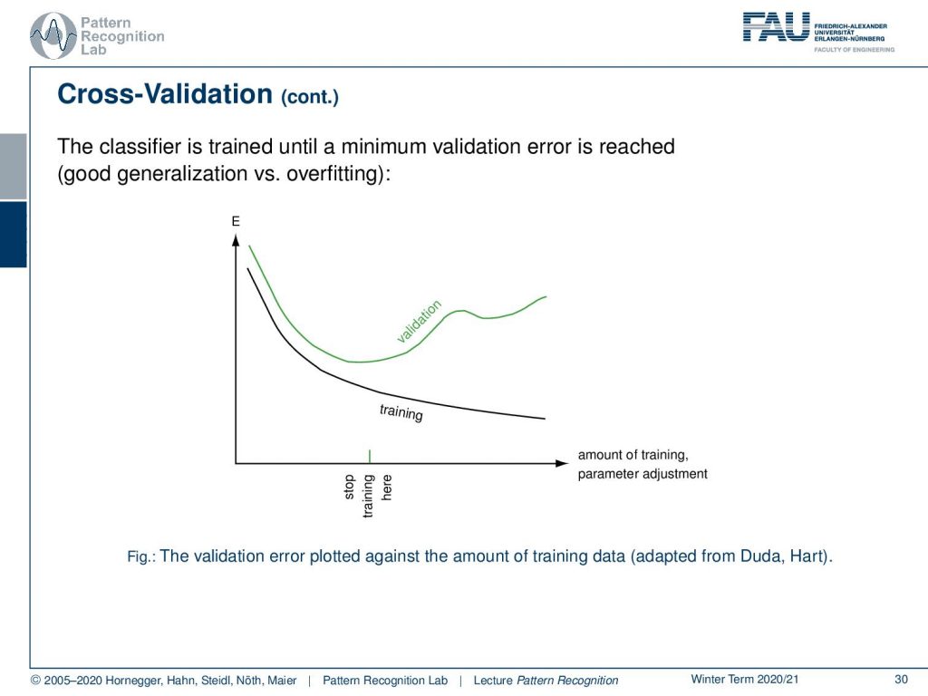
Also what you can do is apply an additional validation set. In this case, you can then determine the parameters that you have to choose during the training process. Let’s say you evaluate your loss on the training set, and then you also look into the validation set. And when you realize that the training loss still is reduced but the validation loss is increased then you may want to stop your training because you’re probably overfitting. Here we have an example. If you run training iterations, of course, because you’re minimizing the loss on the training data will go down and down. But at some time the loss may go up on the validation set, so this would be an appropriate point to stop the entire training process. Know that if you want to apply this in a cross-validation behavior, you have to essentially use m minus two sets for training. One set for validation, and one set for testing. And then you can essentially repeat the procedure also m times.
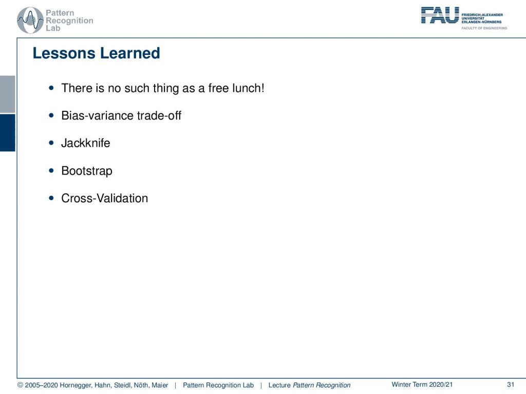
So, what did we learn here? There is no such thing as a free lunch. If you have certain assumptions in a model that are produced by prior knowledge, it may not hold on to a very different classification problem. Generally, there is no best classifier for all the problems. This is the statement of the no free lunch theorem. We’ve also seen that, for a particular problem, we have this biased variance trade-off. So we can increase the capacity of the model and its variance, then we will be able to reduce the bias. But this also comes at the cost that the generalization ability of the model is likely to be reduced in this case. We have seen the Jackknife to estimate out of set performance and to correct for the bias that is introduced by using only a finite set. An alternative is the bootstrap, where the bootstrap is essentially using different sizes of sets and different random sampling. So we can essentially see this as a generalization of the jackknife. And we looked into cross-validation, how to use the Jackknife and bootstrapping principles and how to perform the actual cross-validation to get the estimate for an out of set classification error.

Next time and Pattern Recognition we want to look into one last topic, and this is boosting. and we will introduce the Adaboost principle. You will see that this is a very powerful technique that allows you to combine many weak classification systems into one strong classifier.
I also have some further readings for you. So we’ve seen here Duda and Hart is a very good book. They have very good examples in there. And also Sawyer “Resampling data using a Statistical Jackknife” which is also a very good read. And again, “The Elements of Statistical Learning”.
What you should be able to answer after seeing the last two videos is: What is the meaning of the terms bias and variance? What is the trade-off and how can you estimate the bias and variance of a method if you have only a finite set?
Thank you very much for watching and I’m looking forward to seeing you in the next video! Bye-bye.
If you liked this post, you can find more essays here, more educational material on Machine Learning here, or have a look at our Deep Learning Lecture. I would also appreciate a follow on YouTube, Twitter, Facebook, or LinkedIn in case you want to be informed about more essays, videos, and research in the future. This article is released under the Creative Commons 4.0 Attribution License and can be reprinted and modified if referenced. If you are interested in generating transcripts from video lectures try AutoBlog.
References
- Richard O. Duda, Peter E. Hart, David G. Stork: Pattern Classification, 2nd Edition, John Wiley & Sons, New York, 2000.
- S. Sawyer: Resampling Data: Using a Statistical Jackknife, Washington University, 2005.
- T. Hastie, R. Tibshirani, J. Friedman: The Elements of Statistical Learning, 2nd Edition, Springer, 2009.