
From Class to Pixels
These are the lecture notes for FAU’s YouTube Lecture “Deep Learning“. This is a full transcript of the lecture video & matching slides. We hope, you enjoy this as much as the videos. Of course, this transcript was created with deep learning techniques largely automatically and only minor manual modifications were performed. Try it yourself! If you spot mistakes, please let us know!
Welcome back to deep learning! So, today I want to talk to you about a couple of advanced topics, in particular, looking into sparse annotations. We know that data quality and annotations are extremely costly. In the next couple of videos, we want to talk about some ideas on how to save annotations. The topics will be weakly supervised learning and self-supervised learning.
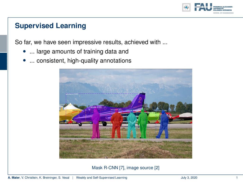
Okay. So, let’s look at our slides and see what I have for you. The topic is weakly and self-supervised learning. We start today by looking into limited annotations and some definitions. Later, we will look into self-supervised learning for representation learning. So, what’s the problem with learning with limited annotations? Well so far. we had supervised learning and we’ve seen these impressive results achieved with large amounts of training data and consistent high-quality annotations. Here, you see an example. We had annotations for instance-based segmentation and there we had simply the assumption that all of these annotations are there. We can use them and there may be even publicly available. So, it’s no big deal. But actually, in most cases, this is not true.
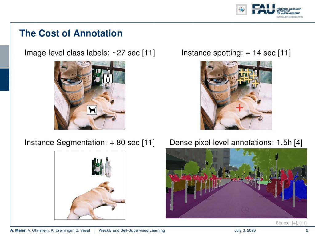
Typically, you have to annotate and annotation is very costly. If you look at image-level class labels, you will spend approximately 20 seconds per sample. So here, you can see for example the image with a dog. There are also ideas where we try to make it faster. For example by instance spotting that you can see here in [11]. If you then go to instance segmentation, you actually have to draw outlines and that’s at least 80 seconds per annotation that you have to spend here. If you go ahead to dense pixel-level annotations, you can easily spend one and a half hours for annotating an image like this one. You can see that in [4].
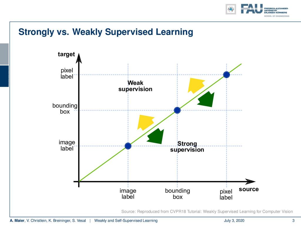
Now, the difference between weakly supervised learning and strong supervision, you can see in this graph. Here, you see that if we have image labels, of course, we can classify image labels and train. That would be essentially supervised learning: Training of bounding boxes to predict bounding boxes and training with pixel labels to predict pixel labels. Of course, you could also abstract from pixel-level labels to bounding boxes or from bounding boxes to image labels. That all would be strong supervision. Now, the idea of weakly supervised learning is that you start with image labels and go to bounding boxes, or you start with bounding boxes and try to predict pixel labels.
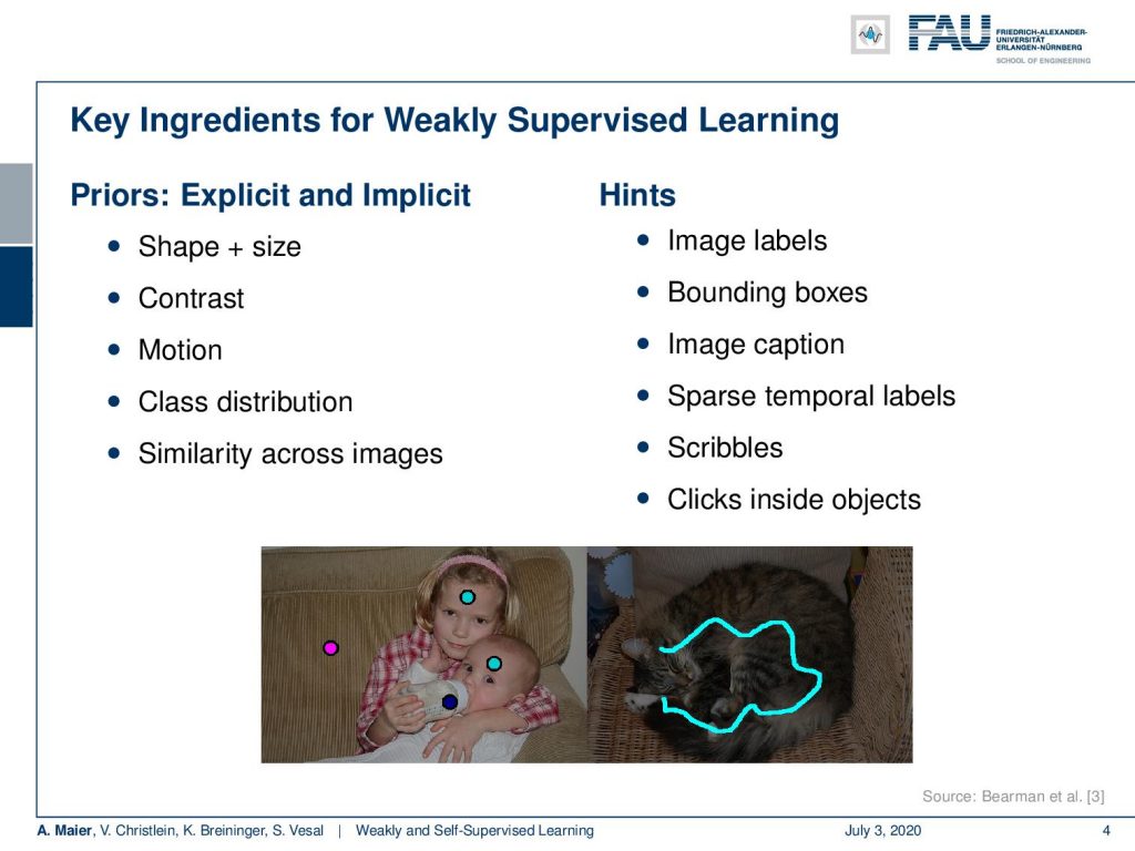
So, this is the key idea in weakly supervised learning. You somehow want to use a sparse annotation and then create much more powerful predictors. The key ingredients for weakly supervised learning are that you use priors. You use explicit and implicit priors about shape, size, and contrast. Also, motion can be used, for example, to shift bounding boxes. The class distributions tell us that some classes are much more frequent than others. Also, similarity across images helps. Of course, you can also use hints like image labels, bounding boxes, and image captions as weakly supervised labels. Sparse temporal labels are propagated over time. Scribbles or clicks inside objects are also suitable. Here, are a couple of examples of such sparse annotations for scribbles and clicks.
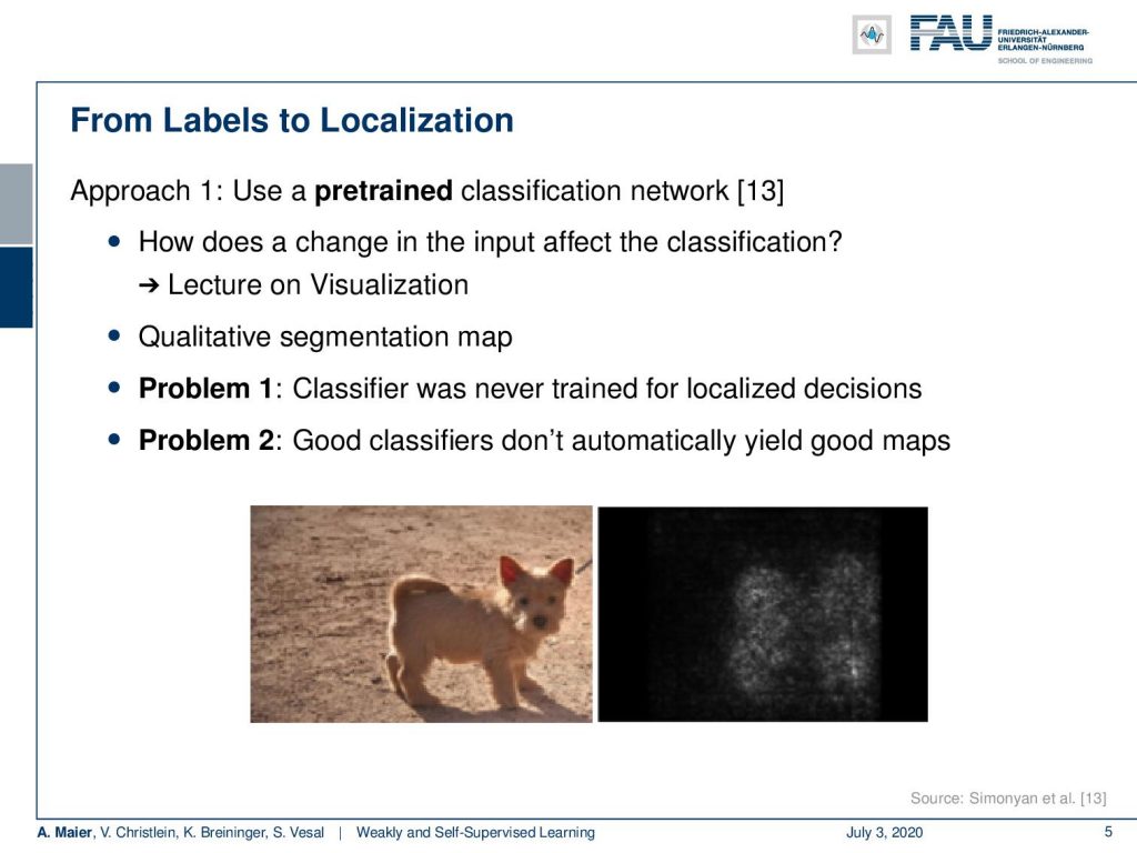
There are some general approaches. One from labels to localization would be that you use a pre-trained classification network. Then, for example, you can use tricks like in the lecture on visualization. You produce a qualitative segmentation map. So here, we had this idea of back-propagating the class label into the image domain in order to produce such labels. Now, the problem is that this classifier was never trained for localized decisions. The second problem is good classifiers don’t automatically yield good maps. So, let’s look into another idea. The key idea here is to use a global average pooling. So let’s rethink the fully convolutional networks and what we’ve been doing there.
You remember that we can replace fully connected layers that have only a fixed input size by M times N convolution. If you do so, we see that if we have some input image and we convolve with a tensor then essentially we get one output. Now, if we have multiple of those tensors then we would essentially get multiple channels. If we now start moving our convolution masks across the image domain, you can see that if we have a larger input image then also our outputs will grow with respect to the output domain. We’ve seen in order to resolve this, we can use global average pooling methods in order to produce the class labels per instance.
Now, what you can do also as an alternative is that you pool first to the correct size. So let’s say, this is your input then you first pool such that you can apply your classification network. Then, go to the classes in a fully connected layer. So, you essentially switch the order of the fully connected layer and the global average pooling. You global average pool first and then produce the classes. We can use this now in order to generate some labels.
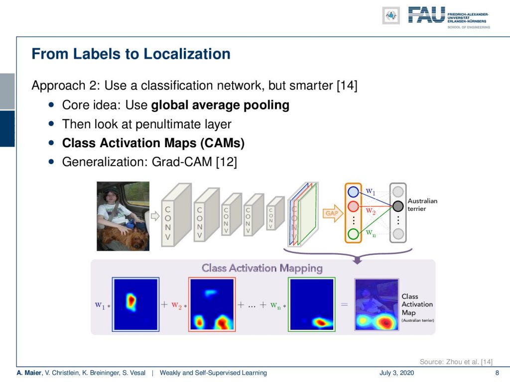
The idea is that now we look at the penultimate layer and we produce class activation maps. So, you see we have two fully connected layers that are producing the class predictions. We have essentially the input feature maps that we can an upscale to the original image size. Then, we use the weights that are assigned to the outputs of the penultimate layer, scale them accordingly, and then produce a class activation map for every output neuron. You can see that here in the bottom happening and by the way there’s also a generalization of this that is then known as Grad-CAM that you can look at in [12]. So with this, we can produce class activation maps and use that as a label for localization.
We can also go from bounding boxes to segmentation. The idea here is that we want to replace an expensively annotated, fully supervised training with bounding boxes because they’re less tedious.
They can be annotated much quicker and of course, this results in a reduced cost. Now, the question is can we use those cheaply annotated labels and weakly supervision in order to produce good segmentations? There is actually a paper out there that looked into this idea.
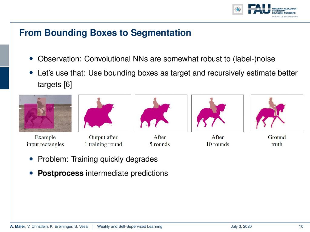
You can see that in [6]. The key idea is that you start with the input rectangles. Then, you do one round of training for a convolutional neural network. You can see that the convolutional neural network is somewhat robust to label noise and therefore if you repeat the process and refine the labels over the iterations, you can see that we get better predictions with each round of training and refining the labels. So on the right-hand side, you see the ground truth and how we gradually approach this. Now, actually there’s a problem because the training very quickly degrades. The only way how you can make this actually work is that you use post-processing in the intermediate predictions.
The idea that they use is that they suppress for example wrong detections. Because you have the bounding boxes, you can be sure that within that bounding box it’s unlikely to have a very different class. Then, you can also essentially remove all the predictions that are outside the bounding box. They are probably not accurate. Furthermore, you can also check if it’s less than a certain percentage of the box area, it’s probably also not an accurate label. In addition, you can use the outside of a conditional random field’s boundaries. We essentially run a kind of traditional segmentation approach to refine the boundary using edge information. You can use that as there’s no information to refine your labels. An additional improvement can be done if you use smaller boxes. On average objects are kind of roundish and therefore the corners and edges contained the least true positives. So, here are some examples of an image, and then you can define regions with unknown labels.
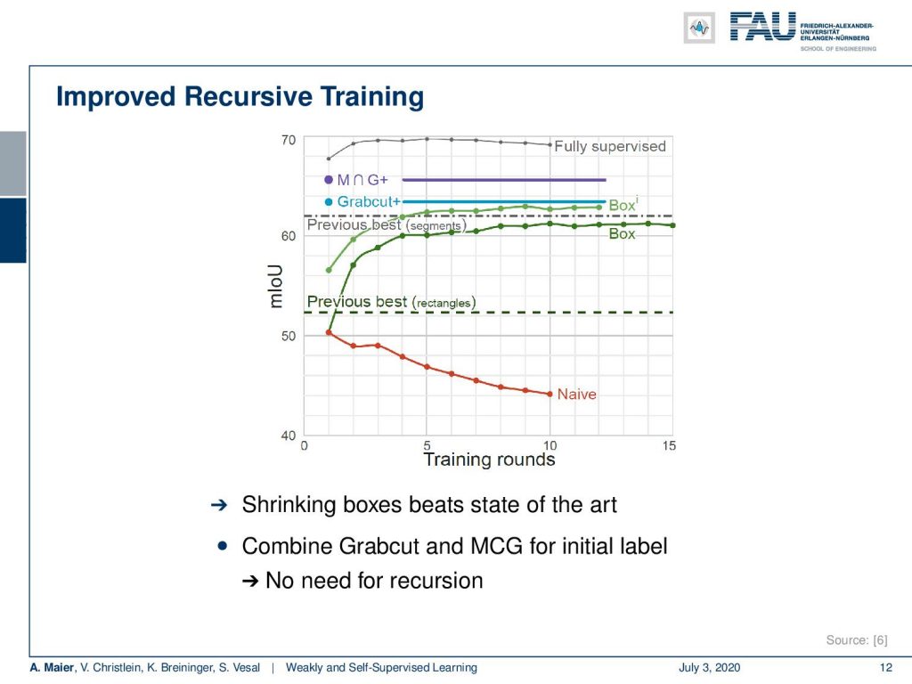
Here are some results. You can see that if we don’t do any refinement of the labels and just train the network over and over again, then you end up in this red line. In the naive approach over the number of training rounds, you actually are reducing the classification accuracy. So the network degenerates and the labels degenerate. That doesn’t work but if you use the tricks with the refinement of the labels with the boxes and excluding outliers, you can actually see that the two green curves emerge. Over the rounds of iterations, you are actually improving. To be honest, if you just use GrabCut+, then you can see that just a single round of iterations is already better than the multiple reruns of the application. If you combine GrabCut+ with the so-called MCG algorithm – the Multi-scale Combinatorial Grouping – you even end up with a better result in just one training round. So, using a heuristic method can also help to improve the labels from bounding boxes to pixel-wise labels. If you look at this, the fully supervised approach is still better. It still makes sense to do the full annotation, but we can already get pretty close in terms of performance if we use one of these weakly supervised approaches. This really depends on your target application. If you’re already ok with let’s say 65% of mean intersection over union then you might be satisfied with the weakly supervised approach. Of course, this is much cheaper than generating the very expensive ground truth annotation.
So next time, we want to continue talking about our weakly-supervised ideas. In the next lecture, we will actually look not just into 2-D images but we’ll also look into volumes and see some smart ideas on how we can use weak annotations in order to generate volumetric 3-D segmentation algorithms. So thank you very much for listening and see you in the next lecture. Bye-bye!
If you liked this post, you can find more essays here, more educational material on Machine Learning here, or have a look at our Deep LearningLecture. I would also appreciate a follow on YouTube, Twitter, Facebook, or LinkedIn in case you want to be informed about more essays, videos, and research in the future. This article is released under the Creative Commons 4.0 Attribution License and can be reprinted and modified if referenced. If you are interested in generating transcripts from video lectures try AutoBlog.
References
[1] Özgün Çiçek, Ahmed Abdulkadir, Soeren S Lienkamp, et al. “3d u-net: learning dense volumetric segmentation from sparse annotation”. In: MICCAI. Springer. 2016, pp. 424–432.
[2] Waleed Abdulla. Mask R-CNN for object detection and instance segmentation on Keras and TensorFlow. Accessed: 27.01.2020. 2017.
[3] Olga Russakovsky, Amy L. Bearman, Vittorio Ferrari, et al. “What’s the point: Semantic segmentation with point supervision”. In: CoRR abs/1506.02106 (2015). arXiv: 1506.02106.
[4] Marius Cordts, Mohamed Omran, Sebastian Ramos, et al. “The Cityscapes Dataset for Semantic Urban Scene Understanding”. In: CoRR abs/1604.01685 (2016). arXiv: 1604.01685.
[5] Richard O. Duda, Peter E. Hart, and David G. Stork. Pattern classification. 2nd ed. New York: Wiley-Interscience, Nov. 2000.
[6] Anna Khoreva, Rodrigo Benenson, Jan Hosang, et al. “Simple Does It: Weakly Supervised Instance and Semantic Segmentation”. In: arXiv preprint arXiv:1603.07485 (2016).
[7] Kaiming He, Georgia Gkioxari, Piotr Dollár, et al. “Mask R-CNN”. In: CoRR abs/1703.06870 (2017). arXiv: 1703.06870.
[8] Sangheum Hwang and Hyo-Eun Kim. “Self-Transfer Learning for Weakly Supervised Lesion Localization”. In: MICCAI. Springer. 2016, pp. 239–246.
[9] Maxime Oquab, Léon Bottou, Ivan Laptev, et al. “Is object localization for free? weakly-supervised learning with convolutional neural networks”. In: Proc. CVPR. 2015, pp. 685–694.
[10] Alexander Kolesnikov and Christoph H. Lampert. “Seed, Expand and Constrain: Three Principles for Weakly-Supervised Image Segmentation”. In: CoRR abs/1603.06098 (2016). arXiv: 1603.06098.
[11] Tsung-Yi Lin, Michael Maire, Serge J. Belongie, et al. “Microsoft COCO: Common Objects in Context”. In: CoRR abs/1405.0312 (2014). arXiv: 1405.0312.
[12] Ramprasaath R. Selvaraju, Abhishek Das, Ramakrishna Vedantam, et al. “Grad-CAM: Why did you say that? Visual Explanations from Deep Networks via Gradient-based Localization”. In: CoRR abs/1610.02391 (2016). arXiv: 1610.02391.
[13] K. Simonyan, A. Vedaldi, and A. Zisserman. “Deep Inside Convolutional Networks: Visualising Image Classification Models and Saliency Maps”. In: Proc. ICLR (workshop track). 2014.
[14] Bolei Zhou, Aditya Khosla, Agata Lapedriza, et al. “Learning deep features for discriminative localization”. In: Proc. CVPR. 2016, pp. 2921–2929.
[15] Longlong Jing and Yingli Tian. “Self-supervised Visual Feature Learning with Deep Neural Networks: A Survey”. In: arXiv e-prints, arXiv:1902.06162 (Feb. 2019). arXiv: 1902.06162 [cs.CV].
[16] D. Pathak, P. Krähenbühl, J. Donahue, et al. “Context Encoders: Feature Learning by Inpainting”. In: 2016 IEEE Conference on Computer Vision and Pattern Recognition (CVPR). 2016, pp. 2536–2544.
[17] C. Doersch, A. Gupta, and A. A. Efros. “Unsupervised Visual Representation Learning by Context Prediction”. In: 2015 IEEE International Conference on Computer Vision (ICCV). Dec. 2015, pp. 1422–1430.
[18] Mehdi Noroozi and Paolo Favaro. “Unsupervised Learning of Visual Representations by Solving Jigsaw Puzzles”. In: Computer Vision – ECCV 2016. Cham: Springer International Publishing, 2016, pp. 69–84.
[19] Spyros Gidaris, Praveer Singh, and Nikos Komodakis. “Unsupervised Representation Learning by Predicting Image Rotations”. In: International Conference on Learning Representations. 2018.
[20] Mathilde Caron, Piotr Bojanowski, Armand Joulin, et al. “Deep Clustering for Unsupervised Learning of Visual Features”. In: Computer Vision – ECCV 2018. Cham: Springer International Publishing, 2018, pp. 139–156. A.
[21] A. Dosovitskiy, P. Fischer, J. T. Springenberg, et al. “Discriminative Unsupervised Feature Learning with Exemplar Convolutional Neural Networks”. In: IEEE Transactions on Pattern Analysis and Machine Intelligence 38.9 (Sept. 2016), pp. 1734–1747.
[22] V. Christlein, M. Gropp, S. Fiel, et al. “Unsupervised Feature Learning for Writer Identification and Writer Retrieval”. In: 2017 14th IAPR International Conference on Document Analysis and Recognition Vol. 01. Nov. 2017, pp. 991–997.
[23] Z. Ren and Y. J. Lee. “Cross-Domain Self-Supervised Multi-task Feature Learning Using Synthetic Imagery”. In: 2018 IEEE/CVF Conference on Computer Vision and Pattern Recognition. June 2018, pp. 762–771.
[24] Asano YM., Rupprecht C., and Vedaldi A. “Self-labelling via simultaneous clustering and representation learning”. In: International Conference on Learning Representations. 2020.
[25] Ben Poole, Sherjil Ozair, Aaron Van Den Oord, et al. “On Variational Bounds of Mutual Information”. In: Proceedings of the 36th International Conference on Machine Learning. Vol. 97. Proceedings of Machine Learning Research. Long Beach, California, USA: PMLR, Sept. 2019, pp. 5171–5180.
[26] R Devon Hjelm, Alex Fedorov, Samuel Lavoie-Marchildon, et al. “Learning deep representations by mutual information estimation and maximization”. In: International Conference on Learning Representations. 2019.
[27] Aaron van den Oord, Yazhe Li, and Oriol Vinyals. “Representation Learning with Contrastive Predictive Coding”. In: arXiv e-prints, arXiv:1807.03748 (July 2018). arXiv: 1807.03748 [cs.LG].
[28] Philip Bachman, R Devon Hjelm, and William Buchwalter. “Learning Representations by Maximizing Mutual Information Across Views”. In: Advances in Neural Information Processing Systems 32. Curran Associates, Inc., 2019, pp. 15535–15545.
[29] Yonglong Tian, Dilip Krishnan, and Phillip Isola. “Contrastive Multiview Coding”. In: arXiv e-prints, arXiv:1906.05849 (June 2019), arXiv:1906.05849. arXiv: 1906.05849 [cs.CV].
[30] Kaiming He, Haoqi Fan, Yuxin Wu, et al. “Momentum Contrast for Unsupervised Visual Representation Learning”. In: arXiv e-prints, arXiv:1911.05722 (Nov. 2019). arXiv: 1911.05722 [cs.CV].
[31] Ting Chen, Simon Kornblith, Mohammad Norouzi, et al. “A Simple Framework for Contrastive Learning of Visual Representations”. In: arXiv e-prints, arXiv:2002.05709 (Feb. 2020), arXiv:2002.05709. arXiv: 2002.05709 [cs.LG].
[32] Ishan Misra and Laurens van der Maaten. “Self-Supervised Learning of Pretext-Invariant Representations”. In: arXiv e-prints, arXiv:1912.01991 (Dec. 2019). arXiv: 1912.01991 [cs.CV].
33] Prannay Khosla, Piotr Teterwak, Chen Wang, et al. “Supervised Contrastive Learning”. In: arXiv e-prints, arXiv:2004.11362 (Apr. 2020). arXiv: 2004.11362 [cs.LG].
[34] Jean-Bastien Grill, Florian Strub, Florent Altché, et al. “Bootstrap Your Own Latent: A New Approach to Self-Supervised Learning”. In: arXiv e-prints, arXiv:2006.07733 (June 2020), arXiv:2006.07733. arXiv: 2006.07733 [cs.LG].
[35] Tongzhou Wang and Phillip Isola. “Understanding Contrastive Representation Learning through Alignment and Uniformity on the Hypersphere”. In: arXiv e-prints, arXiv:2005.10242 (May 2020), arXiv:2005.10242. arXiv: 2005.10242 [cs.LG].
[36] Junnan Li, Pan Zhou, Caiming Xiong, et al. “Prototypical Contrastive Learning of Unsupervised Representations”. In: arXiv e-prints, arXiv:2005.04966 (May 2020), arXiv:2005.04966. arXiv: 2005.04966 [cs.CV].