
Segmentation Basics
These are the lecture notes for FAU’s YouTube Lecture “Deep Learning“. This is a full transcript of the lecture video & matching slides. We hope, you enjoy this as much as the videos. Of course, this transcript was created with deep learning techniques largely automatically and only minor manual modifications were performed. Try it yourself! If you spot mistakes, please let us know!
Welcome back to deep learning! So today, we want to discuss a couple of more application-oriented topics. We want to look into image processing and in particular into segmentation and object detection.
So let’s see what I have here for you. Here’s the outline of the next five videos: We will first introduce the topic, of course. Then, we’ll talk about segmentation. So, we’ll motivate it and discuss where the problems are with segmentation. Then we want to go into several techniques that allow you to do good image segmentation. You will see that there are actually very interesting methods that are quite powerful and can be applied to a wide variety of tasks. After that, we want to continue and talk about object detection. So, this is a kind of related topic. With object detection, we then want to look into different methods of how you can find objects in scenes and how you can actually identify which object belongs to which class. So, let’s start with the introduction.
So far, we looked into image classification. Essentially, you can see that the problem is that you simply have the classification to cat, but you can’t make any information out of the spatial relation of objects to each other. An improvement is image segmentation. So in semantic segmentation, you then try to find the class of every pixel in the image. So here, you can see in red that we marked all of the pixels that belong to the class “cat”. Now, if we want to talk about object detection, we have to look into a slightly different direction. So here, the idea would be to identify essentially the area where the object of interest is. You can already see here if we use for example the methods that we learned in visualization, we will probably not be very happy because we would simply identify pixels that are related to that class. So, this has to be done in a different way because we are actually then interested in finding different instances. So we want to be able to figure out different cats in a single image and then find bounding boxes. So, this is essentially the task of object detection and instance recognition. Now lastly when we have mastered those two ideas, then we also want to talk about the problem of instance segmentation. Here, it’s not just that you find all pixels that show cats but you actually want to differentiate different cats and assign the segmentations to different instances. So, this is then instance segmentation which will be in the last video about these topics.
So, let’s go ahead and talk a bit about ideas towards image segmentation. Now in image segmentation, we want to find exactly which pixels belong to that specific class. We want to delineate essentially the boundary of meaningful objects. So, all of these regions that are within the boundary should have the same label and they belong to the same category. So, each pixel gets a semantic class and we want to generate pixel-wise dense labels. These concepts are, of course, shown here on images but technically you can also do similar things on sound when you, for example, look into spectrograms. The idea in images would be that we want to make out of the left-hand image the right-hand image. You can see already that we find the region that is identified by the airplane here and we find the boundary.
Of course, this is a more simple task. Here, you can also think about more complex scenes like this example here from autonomous driving. Here, we are for example interested in where the street is, where persons are, where pedestrians, where vehicles are, and so on. We want to mark them in this complex scene.
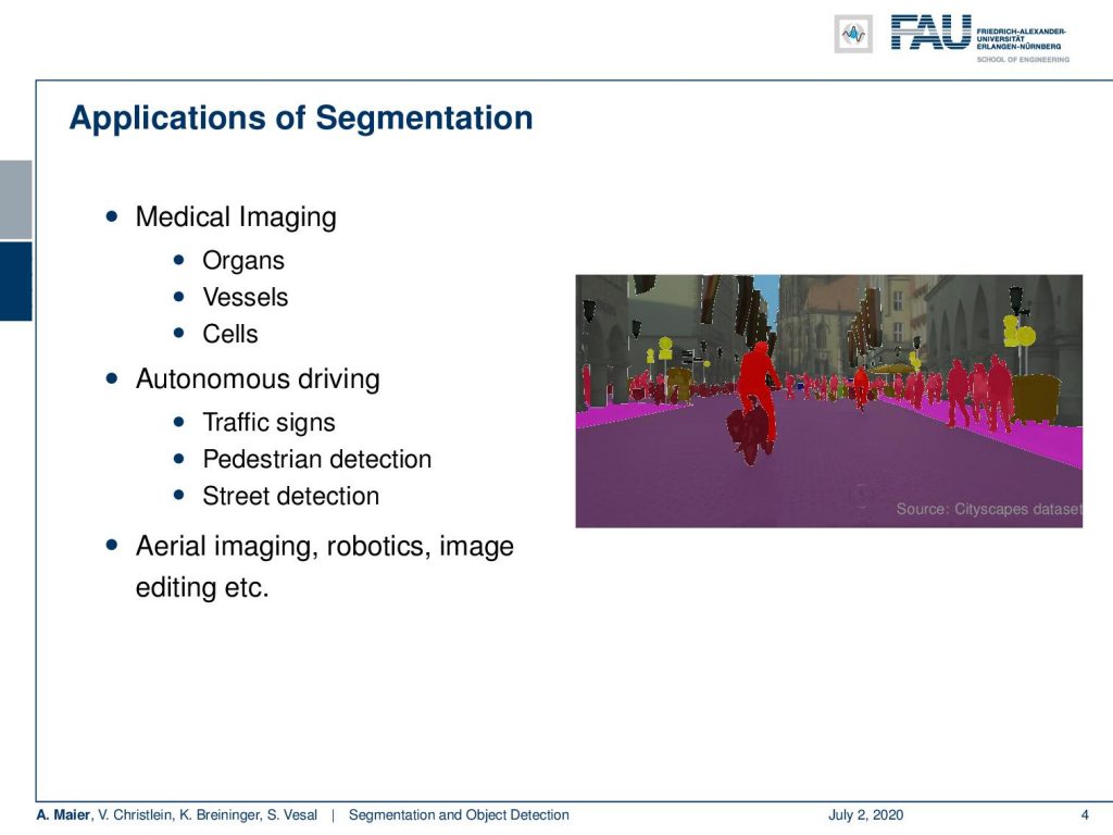
Similar tasks can also be done for medical imaging. For example, if you’re interested in the identification of different organs, i.e., where the liver is, where the vessels are, or where cells are. So, of course, there are many, many more applications that we won’t talk about here. There are aerial images, if you process satellite images, of course, autonomous robotics, and also image editing where you can show that these kinds of techniques have very useful properties.
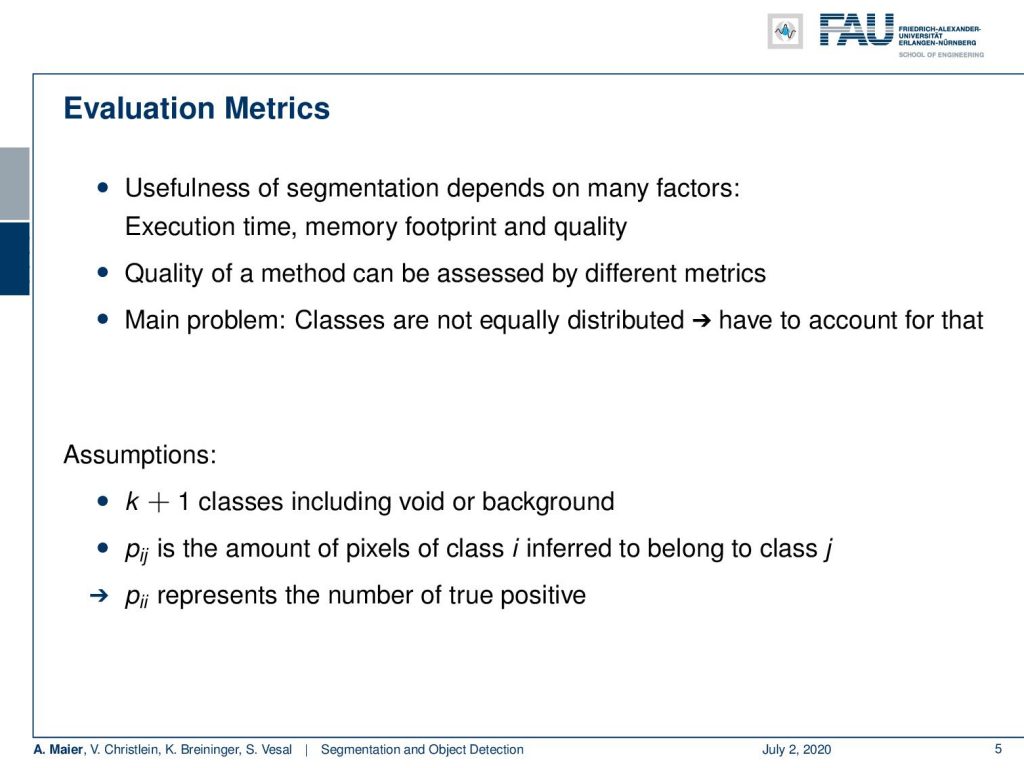
Of course, if we want to do so, we need to talk a bit about evaluation metrics. We have to be somehow able to measure the usefulness of a segmentation algorithm. This depends on several factors like the execution time, memory footprint, and quality. The quality of a method, we need to assess with different metrics. The main problem here is that very often the classes are not equally distributed. So, we have to somehow account for that. We can do that by also expanding the number of classes with a background class. Then, we can determine, for example, the probability of the pixel of class i to be inferred to belong to class j. For example, p subscript i, i would then represent the number of true positives.
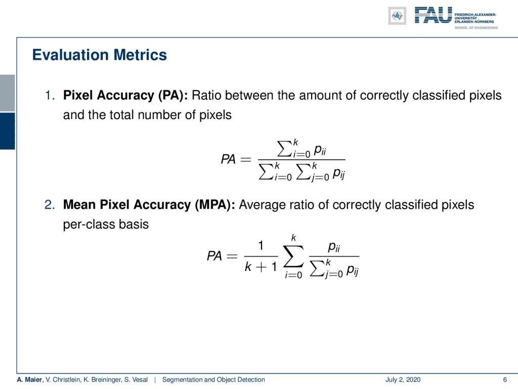
This then brings us to several metrics, for example, the pixel accuracy that would be the ratio between the amount of correctly classified pixels and the total number of pixels and the mean pixel accuracy which is the average ratio of correctly classified pixels per class basis.
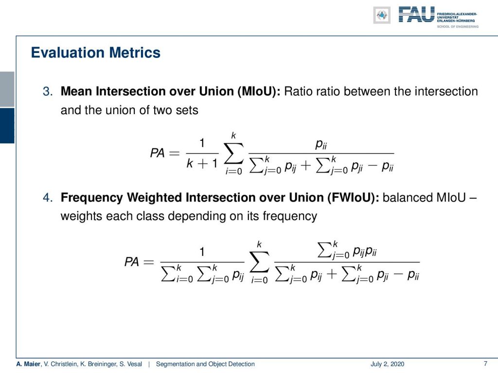
More common actually to evaluate segmentations are then things like the mean intersection over union which is then the ratio between the intersection and the union of two sets and the frequency weighted intersection of a union which is then a balanced version where you also incorporate the class frequency into this measure. So, with these measures then we can figure out what a good segmentation is.
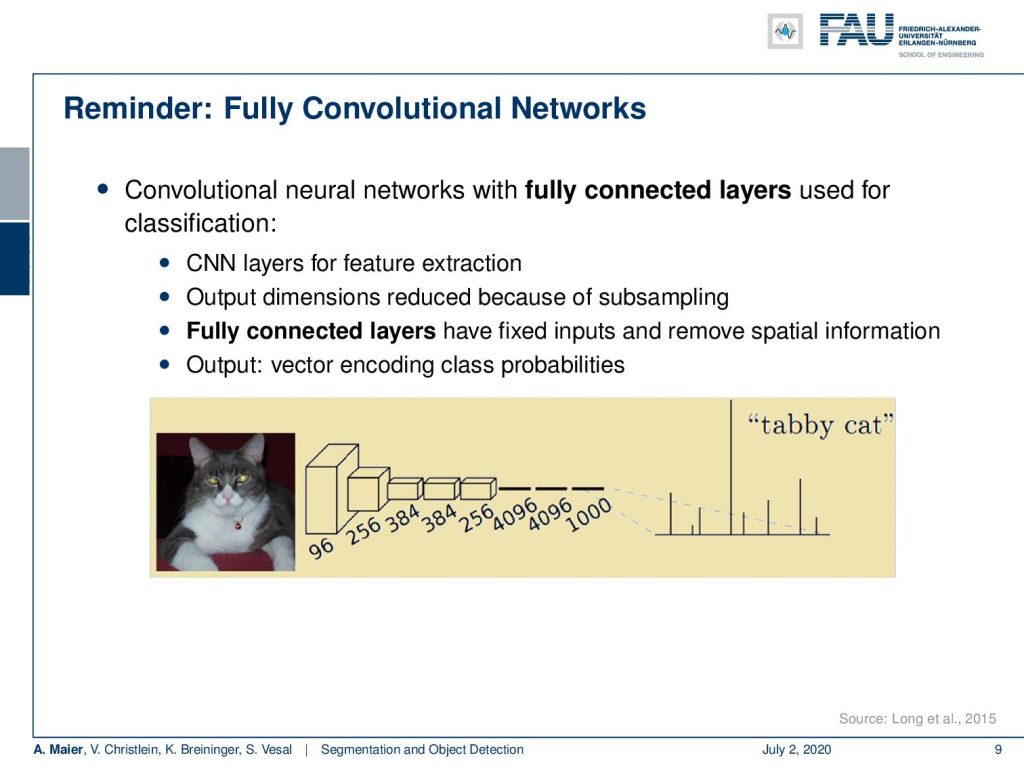
Then, we go ahead and, of course, we follow the ideas of using fully convolutional networks for segmentation. Now so far, if we have been using fully convolutional networks, we essentially had a high-dimensional input – the image – and then we used this CNN for the feature extraction. Then, the outputs were essentially the distributions over different classes. Thus, we had essentially a vector encoding the class probabilities.
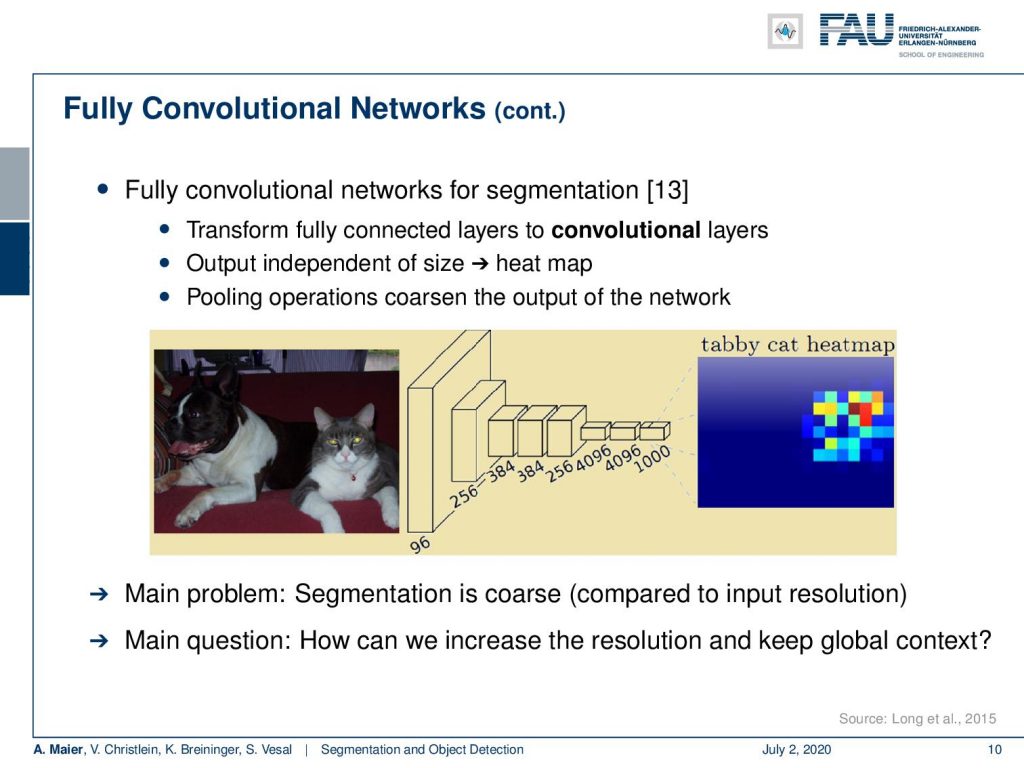
So, you could also transform it into a fully convolutional neural network where you then essentially parse the entire image and transform it into a heat map. So, we’ve seen similar ideas already in visualization when we talked about the different activations. We could essentially also follow this line of interpretation and then we would get a very low dimensional very coarse heat map for the class “tabby cat”. This is, of course, one way it can go, but you will not be able to identify all the pixels that belong to that specific class in great detail. So, what you have to do is you somehow have to get the segmentation or the class information back to the original image resolution.
Here, the key idea is not just to use a CNN as an encoder, but you also use a decoder. So, we end up with a structure that looks like this kind of CNN – you could even say hourglass – where we have this encoder and a decoder that does the upsampling again. This is, by the way, not an autoencoder because the input is the image, but the output is the segmentation mask. The encoder part of the network is essentially a CNN and this is very similar to techniques that we already talked about quite a bit.
So, on the other side, we need a decoder. This decoder then is used to upsample the information again. There are actually several approaches on how to do this. One of the early ones is Long et al.’s Fully Convolutional Network [13]. There’s also SegNet [1] and I think the most popular one is U-net [21]. This is also the paper that I hinted at that has the many references. So, U-net is really popular and you can see that you can check the citation count every day.
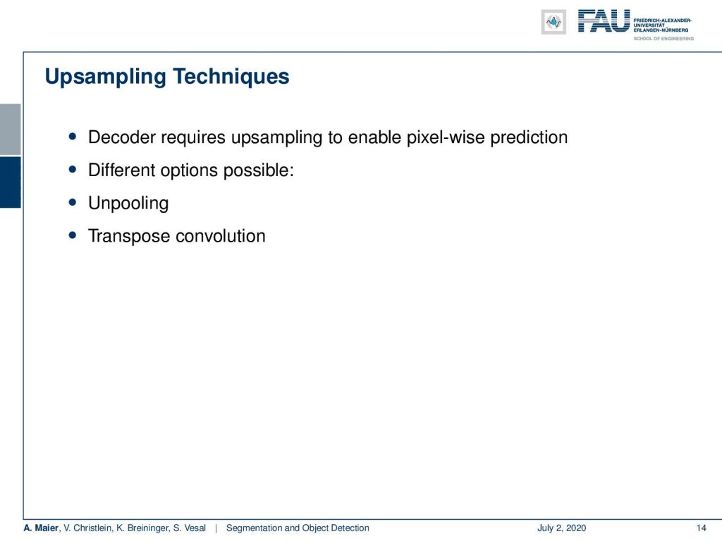
Well, let’s discuss how we can do this. The main issue is the upsampling part. So here, we want to have a decoder that somehow is creating a pixel-wise prediction. There are different options possible and one is, for example, unpooling. You can also do transpose convolutions which essentially is then not using the idea of pooling, but the idea of convolution but transposed such that you increase the resolution instead of doing a subsampling.
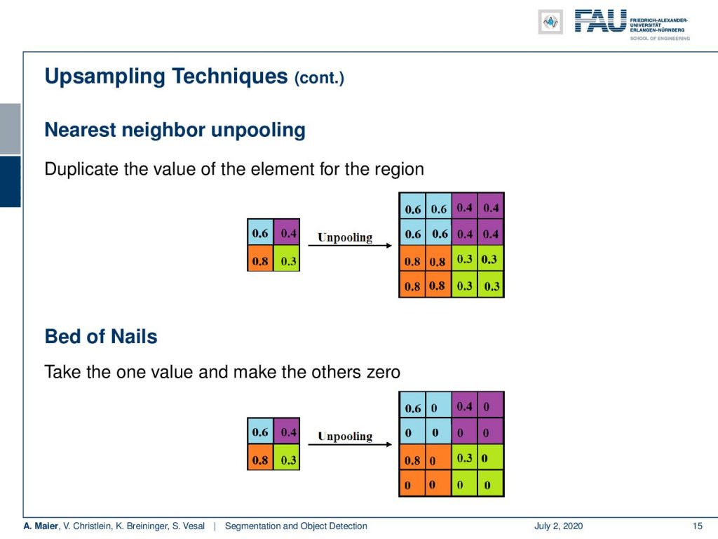
So, let’s look at those upsampling techniques in some more detail. Of course, you can do something like the nearest-neighbor interpolation. There you then simply take the low-resolution information and you unpool simply by taking the nearest neighbor. There’s the bed of nails on which then takes just a single value and you just put it at one of the locations. So, the remaining image will look like a bed of nails. The idea here is, of course, that you just put the information at the position where you know that it belongs. Then, the remaining missing entries should be filled up by a learnable part that is then introduced in a later step of this network.
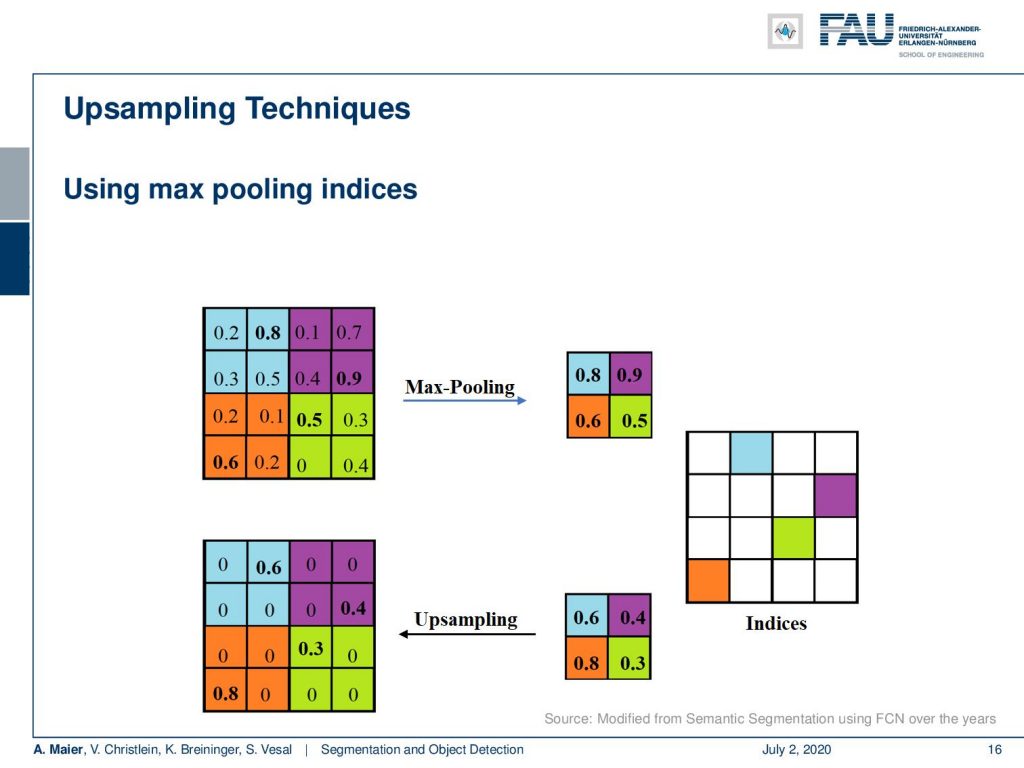
Another approach is using max-pooling indices. So, here the idea is that in the encoder path, you perform max pooling and you save the indices of where the pooling actually occurred. Then, you can take this information in the upsampling step again and you write the information exactly at the place where the maximum came from. So this is very similar to what you would be doing in the backpropagation step of the maximum pooling.
Of course, there are also learnable techniques like the transposed convolution. Here, you learn an upsampling which is then sometimes also called deconvolution. What you actually do is you have a filter that moves essentially two pixels in the output for every one pixel in the input. You can control higher upsampling with the stride. So, let’s look at this example here. We have this single pixel that then gets unpooled. Here, you produce this 3 x 3 transpose convolution. We show it with a stride of two. Then, we move to the next pixel and you can see that an overlap area emerges in this case. There, you have to do something about this overlap area. For example, you could simply sum them up and hope that in the subsequent processing your network learns how to deal with this inconsistency in the upsampling step.
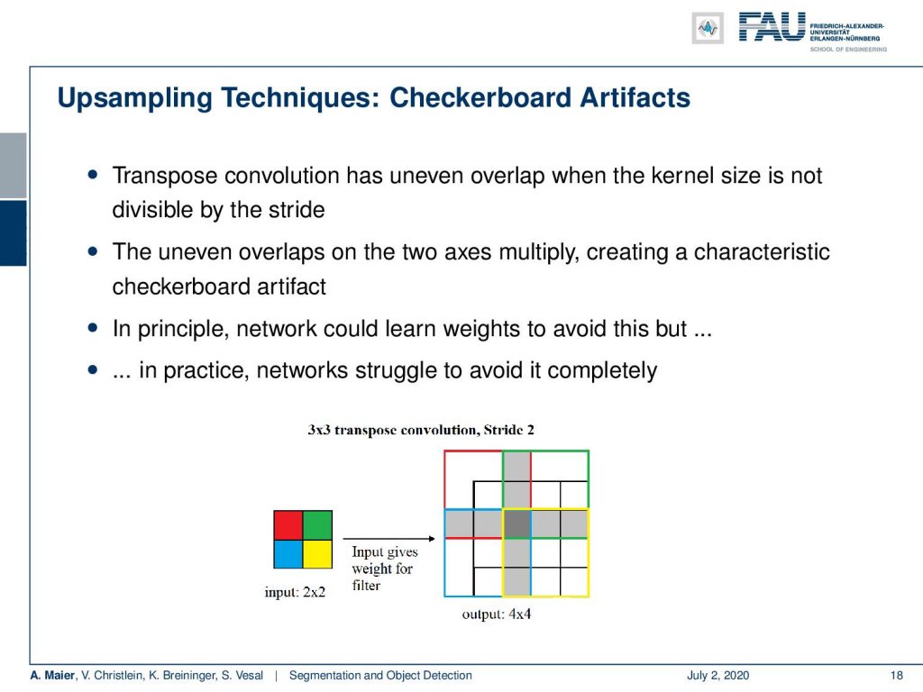
We can go ahead and do this for the other two pixels in this example. Then, you see that we have this cross-shaped area. So, the transpose convolution results in an uneven overlap when the kernel size is not divisible by the stride. These uneven overlaps on the axis multiply and they create this characteristic checkerboard artifact. In principle, as mentioned before you should be able to learn how to remove those artifacts again in subsequent layers. In practice, it causes struggle and we recommend to avoid it completely.
So, how can this be avoided? Well, you choose an appropriate kernel size. You choose the kernel size in a way that it is divisible by the stride. Then, you can also do separate upsampling from convolution to compute the features. For example, you could resize the image using a neural network or by linear interpolation. Then, you add a convolution layer. So, this would be a typical approach to do this.
Okay. So until now, we understood all of the basic steps that we need in order to perform image segmentation. Actually, in the next video, we will then talk about how to actually integrate the encoder and the decoder to get good segmentation masks. I may already tell you, there’s a specific trick that you have to do. If you don’t use this trick, you will probably not be able to get a very good segmentation result. So, please stay tuned for the next video because there you will see how you can do good segmentations. You will learn about all the details of these advanced segmentation techniques. So thank you very much for listening and see you in the next video. Bye-bye!
If you liked this post, you can find more essays here, more educational material on Machine Learning here, or have a look at our Deep LearningLecture. I would also appreciate a follow on YouTube, Twitter, Facebook, or LinkedIn in case you want to be informed about more essays, videos, and research in the future. This article is released under the Creative Commons 4.0 Attribution License and can be reprinted and modified if referenced. If you are interested in generating transcripts from video lectures try AutoBlog.
References
[1] Vijay Badrinarayanan, Alex Kendall, and Roberto Cipolla. “Segnet: A deep convolutional encoder-decoder architecture for image segmentation”. In: arXiv preprint arXiv:1511.00561 (2015). arXiv: 1311.2524.
[2] Xiao Bian, Ser Nam Lim, and Ning Zhou. “Multiscale fully convolutional network with application to industrial inspection”. In: Applications of Computer Vision (WACV), 2016 IEEE Winter Conference on. IEEE. 2016, pp. 1–8.
[3] Liang-Chieh Chen, George Papandreou, Iasonas Kokkinos, et al. “Semantic Image Segmentation with Deep Convolutional Nets and Fully Connected CRFs”. In: CoRR abs/1412.7062 (2014). arXiv: 1412.7062.
[4] Liang-Chieh Chen, George Papandreou, Iasonas Kokkinos, et al. “Deeplab: Semantic image segmentation with deep convolutional nets, atrous convolution, and fully connected crfs”. In: arXiv preprint arXiv:1606.00915 (2016).
[5] S. Ren, K. He, R. Girshick, et al. “Faster R-CNN: Towards Real-Time Object Detection with Region Proposal Networks”. In: vol. 39. 6. June 2017, pp. 1137–1149.
[6] R. Girshick. “Fast R-CNN”. In: 2015 IEEE International Conference on Computer Vision (ICCV). Dec. 2015, pp. 1440–1448.
[7] Tsung-Yi Lin, Priya Goyal, Ross Girshick, et al. “Focal loss for dense object detection”. In: arXiv preprint arXiv:1708.02002 (2017).
[8] Alberto Garcia-Garcia, Sergio Orts-Escolano, Sergiu Oprea, et al. “A Review on Deep Learning Techniques Applied to Semantic Segmentation”. In: arXiv preprint arXiv:1704.06857 (2017).
[9] Bharath Hariharan, Pablo Arbeláez, Ross Girshick, et al. “Simultaneous detection and segmentation”. In: European Conference on Computer Vision. Springer. 2014, pp. 297–312.
[10] Kaiming He, Georgia Gkioxari, Piotr Dollár, et al. “Mask R-CNN”. In: CoRR abs/1703.06870 (2017). arXiv: 1703.06870.
[11] N. Dalal and B. Triggs. “Histograms of oriented gradients for human detection”. In: 2005 IEEE Computer Society Conference on Computer Vision and Pattern Recognition Vol. 1. June 2005, 886–893 vol. 1.
[12] Jonathan Huang, Vivek Rathod, Chen Sun, et al. “Speed/accuracy trade-offs for modern convolutional object detectors”. In: CoRR abs/1611.10012 (2016). arXiv: 1611.10012.
[13] Jonathan Long, Evan Shelhamer, and Trevor Darrell. “Fully convolutional networks for semantic segmentation”. In: Proceedings of the IEEE Conference on Computer Vision and Pattern Recognition. 2015, pp. 3431–3440.
[14] Pauline Luc, Camille Couprie, Soumith Chintala, et al. “Semantic segmentation using adversarial networks”. In: arXiv preprint arXiv:1611.08408 (2016).
[15] Christian Szegedy, Scott E. Reed, Dumitru Erhan, et al. “Scalable, High-Quality Object Detection”. In: CoRR abs/1412.1441 (2014). arXiv: 1412.1441.
[16] Hyeonwoo Noh, Seunghoon Hong, and Bohyung Han. “Learning deconvolution network for semantic segmentation”. In: Proceedings of the IEEE International Conference on Computer Vision. 2015, pp. 1520–1528.
[17] Adam Paszke, Abhishek Chaurasia, Sangpil Kim, et al. “Enet: A deep neural network architecture for real-time semantic segmentation”. In: arXiv preprint arXiv:1606.02147 (2016).
[18] Pedro O Pinheiro, Ronan Collobert, and Piotr Dollár. “Learning to segment object candidates”. In: Advances in Neural Information Processing Systems. 2015, pp. 1990–1998.
[19] Pedro O Pinheiro, Tsung-Yi Lin, Ronan Collobert, et al. “Learning to refine object segments”. In: European Conference on Computer Vision. Springer. 2016, pp. 75–91.
[20] Ross B. Girshick, Jeff Donahue, Trevor Darrell, et al. “Rich feature hierarchies for accurate object detection and semantic segmentation”. In: CoRR abs/1311.2524 (2013). arXiv: 1311.2524.
[21] Olaf Ronneberger, Philipp Fischer, and Thomas Brox. “U-net: Convolutional networks for biomedical image segmentation”. In: MICCAI. Springer. 2015, pp. 234–241.
[22] Kaiming He, Xiangyu Zhang, Shaoqing Ren, et al. “Spatial Pyramid Pooling in Deep Convolutional Networks for Visual Recognition”. In: Computer Vision – ECCV 2014. Cham: Springer International Publishing, 2014, pp. 346–361.
[23] J. R. R. Uijlings, K. E. A. van de Sande, T. Gevers, et al. “Selective Search for Object Recognition”. In: International Journal of Computer Vision 104.2 (Sept. 2013), pp. 154–171.
[24] Wei Liu, Dragomir Anguelov, Dumitru Erhan, et al. “SSD: Single Shot MultiBox Detector”. In: Computer Vision – ECCV 2016. Cham: Springer International Publishing, 2016, pp. 21–37.
[25] P. Viola and M. Jones. “Rapid object detection using a boosted cascade of simple features”. In: Proceedings of the 2001 IEEE Computer Society Conference on Computer Vision Vol. 1. 2001, pp. 511–518.
[26] J. Redmon, S. Divvala, R. Girshick, et al. “You Only Look Once: Unified, Real-Time Object Detection”. In: 2016 IEEE Conference on Computer Vision and Pattern Recognition (CVPR). June 2016, pp. 779–788.
[27] Joseph Redmon and Ali Farhadi. “YOLO9000: Better, Faster, Stronger”. In: CoRR abs/1612.08242 (2016). arXiv: 1612.08242.
[28] Fisher Yu and Vladlen Koltun. “Multi-scale context aggregation by dilated convolutions”. In: arXiv preprint arXiv:1511.07122 (2015).
[29] Shuai Zheng, Sadeep Jayasumana, Bernardino Romera-Paredes, et al. “Conditional Random Fields as Recurrent Neural Networks”. In: CoRR abs/1502.03240 (2015). arXiv: 1502.03240.
[30] Alejandro Newell, Kaiyu Yang, and Jia Deng. “Stacked hourglass networks for human pose estimation”. In: European conference on computer vision. Springer. 2016, pp. 483–499.