Lecture Notes in Deep Learning: Introduction – Part 4

A short course in Pattern Recognition

These are the lecture notes for FAU’s YouTube Lecture “Deep Learning“. This is a full transcript of the lecture video & matching slides. We hope, you enjoy this as much as the videos. Of course, this transcript was created with deep learning techniques largely automatically and only minor manual modifications were performed. If you spot mistakes, please let us know!

Welcome to our deep learning lecture. We are now in Part 4 of the introduction. Now, in this fourth path we want to talk about machine learning and pattern recognition and first of all we have to introduce a bit of terminology and notation.

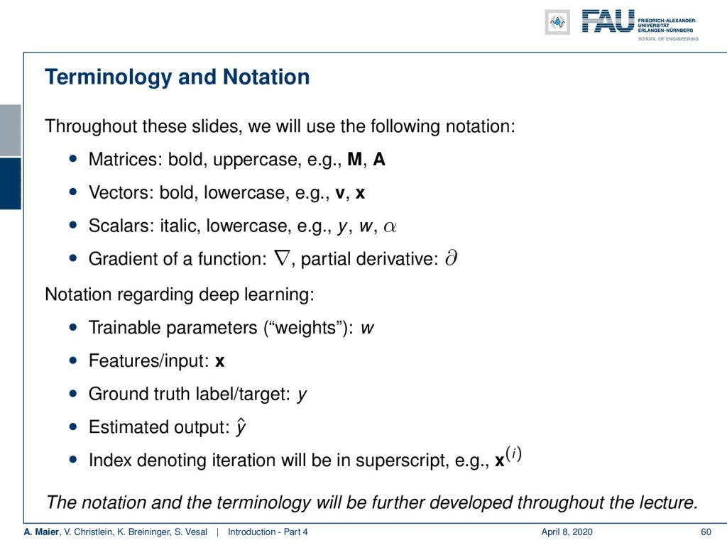
So, throughout this entire lecture series, we will use the following notation: Matrices are bold and uppercase. So, examples here are M and A. Vectors are bold and lowercase examples are v and x. Scalars are italic and lowercase: y, w, α. For the gradient of a function, we use the gradient symbol ∇, for partial derivatives we use the partial notation ∂. Furthermore, we have some specifics about deep learning. So, the trainable weights will generally be called w. Features or inputs are x. They are typically vectors. Then, we have the ground truth label which is y. We have some estimated output that is 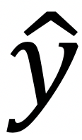and if we have some iterations going on, we typically do that in superscript and put it into brackets. This is an iteration index here: Iteration i for variable x. Of course, this is a very coarse notation and we will develop it further throughout the lecture.

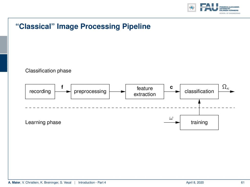
If you have attended previous lectures of our group, then you should know the classical image processing pipeline of pattern recognition. It does recording with sampling followed by analog to digital conversion.Then, you have the pre-processing, feature extraction followed by classification. Of course, in the classification step, you have to do the training. The first part of the pattern recognition pipeline is covered in our lecture introduction pattern recognition. The main part of classification is covered in pattern recognition.

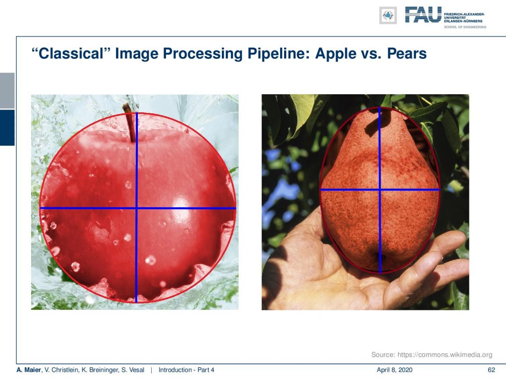
Now, what you see in this image is a classical image recognition problem. Let’s say, you want to differentiate apples from pears. Now, one idea that you could do is you could draw a circle around them and then measure the length of the major and minor axes. So, you will recognize that apples are round and pears are longer. So, their ellipses have a difference in the major and minor axis.

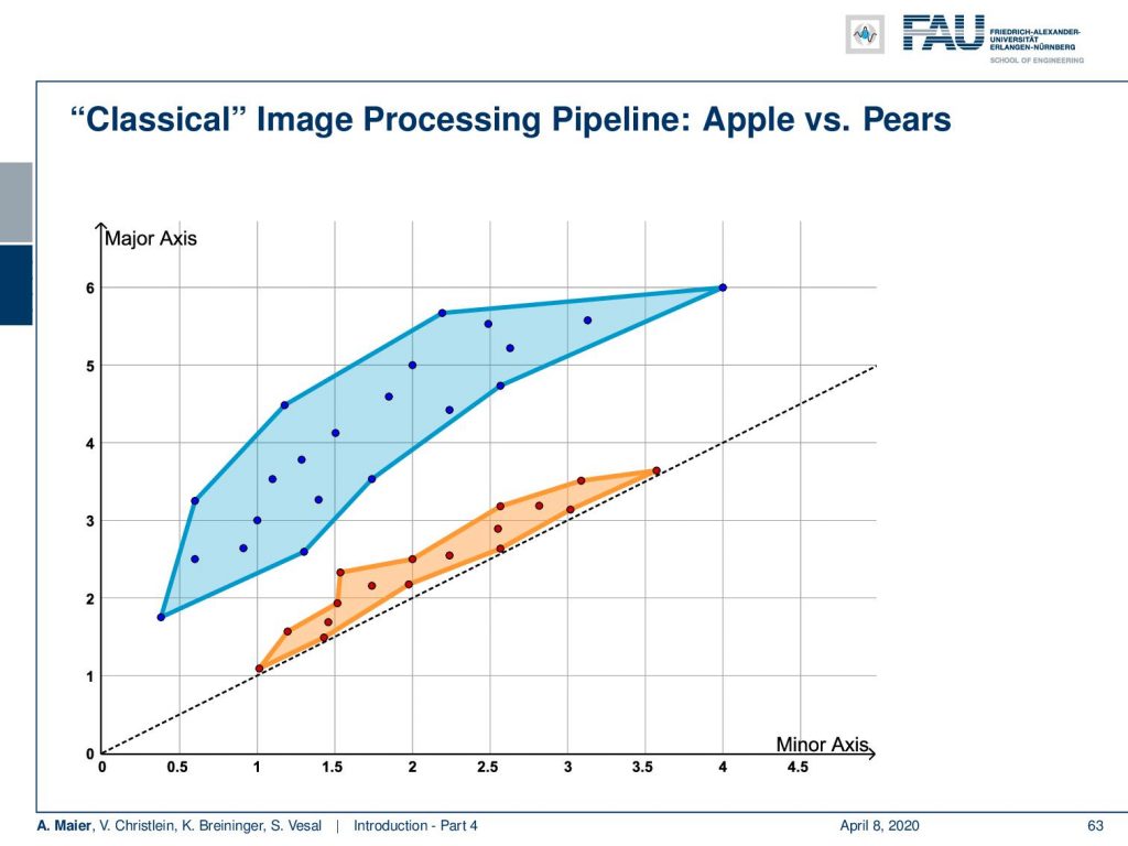
Now, you could take those two numbers and represent them as a vector value. Then, you enter a two-dimensional space which is basically a vector space representation in which you will find that all of the apples are located on the diagonal through the x-axis. If their diameter and one direction increases, also the diameter and the other direction increases. Your pears are off this straight line because they have a difference in their minor and major axes. Now, you can find a line that separates those two and there you have your first classification system.

Now, what many people think about how the big data processing works is shown in this small figure:

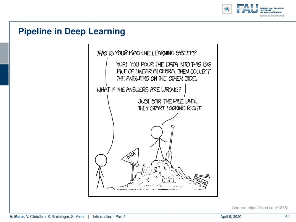
So, what you can see in this picture is that of course this is how many people think that they approach deep learning. You just pour the data in and in the end you just stir a bit and then you get the right results.

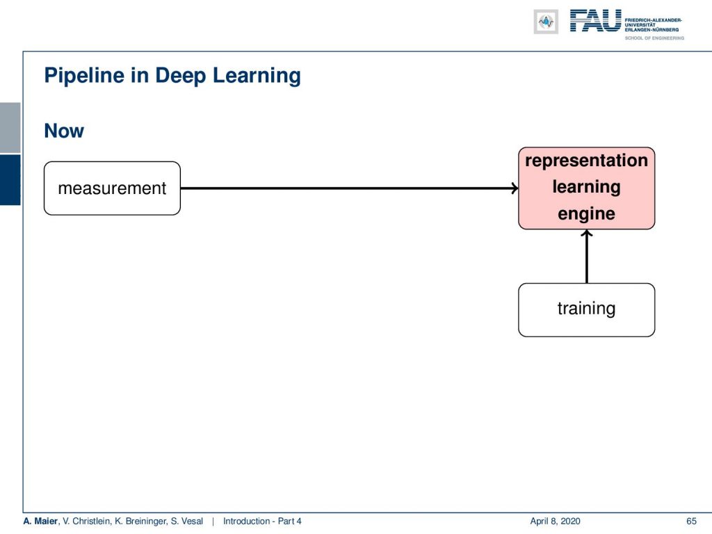
But that’s not actually how it works. Remind them what you want to do is you want to build a system that learns a classification. This means that from your measurement you first have to do some pre-processing like reduce noise. You have to get a meaningful image then do feature extraction and from that, you can then do a classification. Now, the difference to deep learning is that you put everything into a single kind of engine. So, this does the pre-processing, the feature extraction, and the classification just in a single step. You just use the training data and the measurement in order to produce those systems. Now, this has been shown to work in a lot of applications, but as we’ve already talked about in the last video, you have to have the right data. You cannot just pour some data in and then stir until it starts looking right. You have to have a proper data set, a proper data collection, and if you don’t do that in the appropriate way, you just get nonsense.

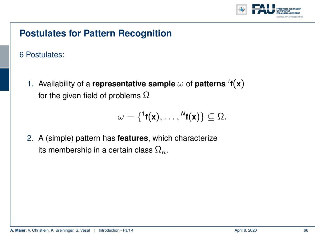
Of course, we have a couple of postulates and those postulates also apply in the regime of deep learning. So in classical pattern recognition, we are following those postulates. So, the first postulate is that there’s a variability of representative sampling patterns and those sampling patterns are given in the class and the problem domain Omega. Here, you have training examples for all of those classes and they are representative. So, it means that if you have a new observation, it will be similar to those patterns that you already collected. The next postulate is that there is a simple pattern and the simple pattern has features that characterize the membership to a certain class. So, you have to somehow be able to process the data to derive this abstract representation. With this representation, you can then derive the class in the classifier.

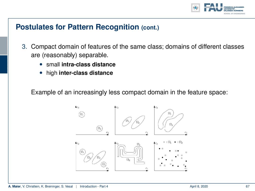
Furthermore, features of the same class should be compact in the feature domain. So, this means that features of different classes, they should be apart from other classes while features of the same class should be close to each other. So, what you want to have ideally is a small intraclass variance and a high inter-class distance. Examples are shown here in this figure. So the top left one is a very nice and easy example. The one in the center is also solvable. It gets harder for the third one and of course, you can still separate them by a nonlinear boundary. More complicated is the case on the bottom left because here the classes are intermixed and you want to essentially draw regions around those classes. They may also be very intertwined but still separable and then of course you could have data where it’s very hard to figure out which part goes to where. Typically if you have a situation like the bottom right, you don’t have a very good feature representation and you want to think whether you don’t find better features. What many people do today is they just say: “Oh, let’s go to deep learning and just learn an appropriate representation that then will do the trick.”

So, a complex pattern consists of simpler constituents that have a certain relation to each other and the pattern may be decomposed into those parts. Furthermore, a complex pattern has a certain structure and not every arrangement of simpler parts gives a valid pattern and many patterns can be represented with relatively few parts. Of course, two patterns are similar if the features of simpler parts differ only slightly. Having seen those basic postulates of pattern recognition, we will see that many of them still apply also in the world of deep learning. However, we don’t see really how things are decomposed. Instead, we build systems that gradually simplify the input such that you decompose them into parts and better representations.

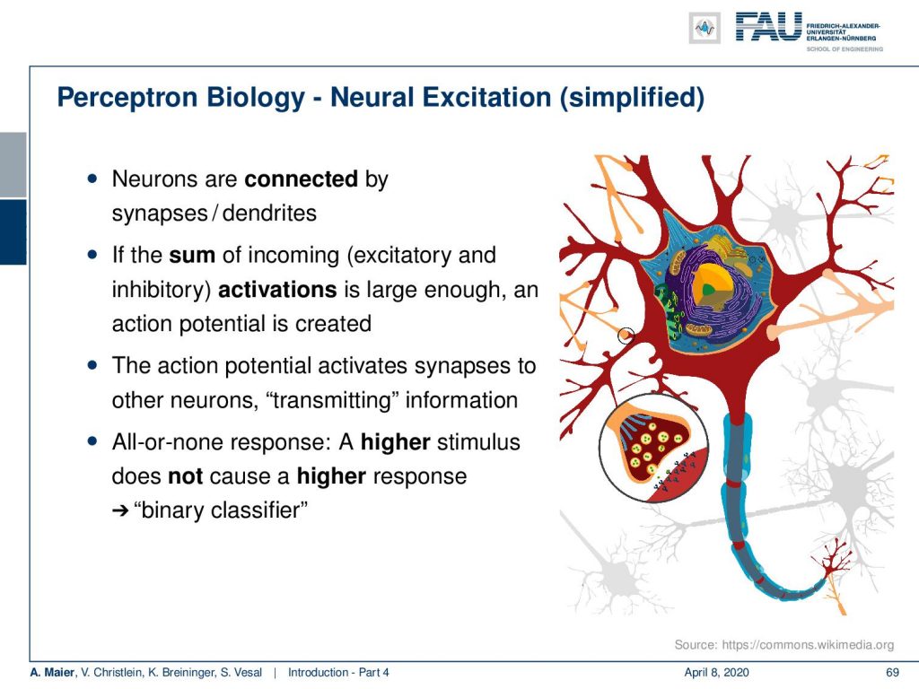
Now, let’s start with the very basics. The perceptron is the basic unit that you will find in most neural networks and the reason why people are very excited about perceptrons. Actually, when they are introduced by Rosenblatt in the 1950s, they people got really excited because Rosenblatt had this nice relation of this perceptron to a biological neuron. Now, a biological neuron is connected by synapses to other neurons and compute the sum of incoming excitatory and inhibitory activations. If they are large enough, then the neuron is firing and it’s firing if you have a certain potential that is over a threshold. Then, it’s transmitting information and it’s typically an all-or-none response which means that if you have a higher stimulus and you exceed the threshold, it doesn’t mean that it causes a higher response. It either fires or doesn’t fire. So it’s essentially a binary classifier.

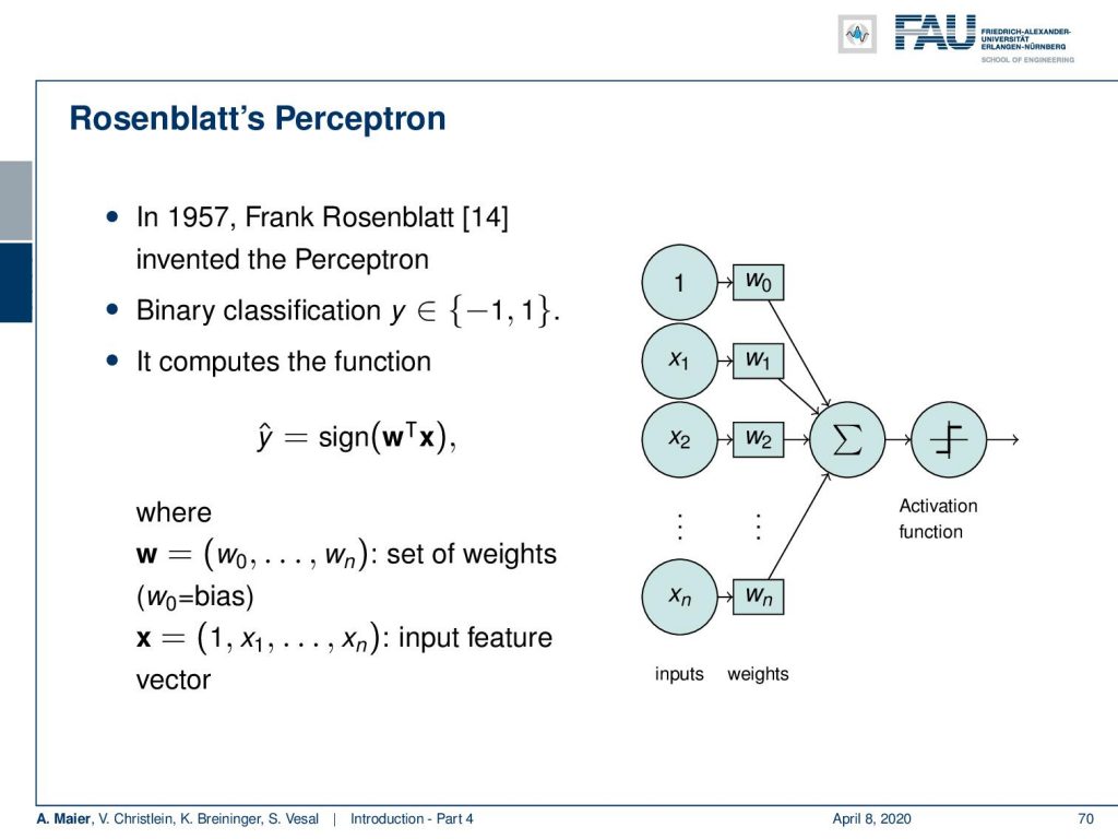
This concept can rather easily be transformed into a vector representation. He essentially devised a system that takes an input vector that is specified here by input values x₁ to and you added some bias one. Here, you multiply them with weights add them up. Then, you have an activation function that either fires but doesn’t, and here for a sake of simplicity, we can simply take the sign function. So, if you have a positive activation, you fire. If you have a negative activation, you don’t fire. So, this could be represented by the sign function. Now, this then leads to a rather problematic training procedure.

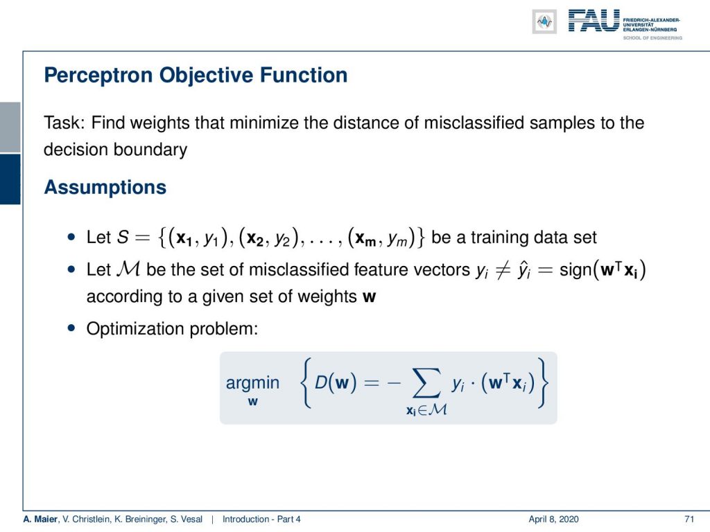
Of course, if you want to train, you need to have tuples of observations of the respective classes. This is your training data set and then you need to determine the set M of the misclassified feature vectors. So, these are the vectors where the predicted number does not match the actual class membership yᵢ. if you compute the output of the neuron. Now, if you have this set M that has to be determined after each step of the training iteration, then you try to minimize the following optimization problem: The problem that describes your misclassification is essentially the sum of all your misclassified samples where you compute the output of your actual neuron. This is then multiplied by the true class membership. So because the two don’t match, it means this must be negative. Then, you multiply above term with minus 1, in order to create a high value for a lot of misclassifications. You seek to minimize this term.

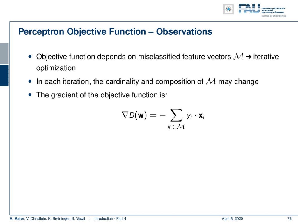
This essentially then leads to an optimization procedure where you have an iterative procedure. So, this iterative optimization then has to determine an updated gradient step for the weights. Once you update the weights, you have to determine the set of misclassified vectors again. Now, the problem with this is that in every iteration the cardinality of the composition of M may change because with every step you have more of your misclassifications. You actually compute the gradient of the function with respect to the weights and it’s simply the input vector multiplied with the correct class minus one. This will give you an update on the weight.

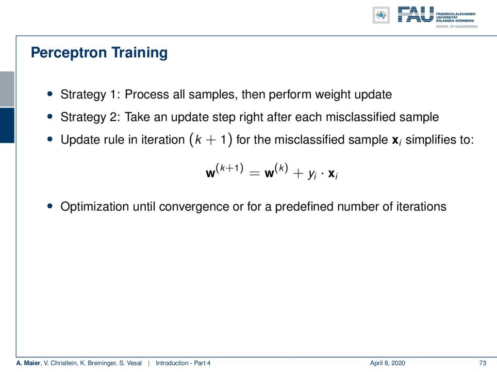
Now, if you calculated this gradient, Strategy 1 would be processing all of the samples and then perform the weight update. Strategy 2 is to take an update step after each missing classified sample and then directly update weights. So, you get an update rule for each iteration which simplifies to: The old weights plus the misclassified sample multiplied with the class membership. This gives you the new weights. Now, you optimize onto convergence or for a predefined number of iterations. This very simple procedure has a number of disadvantages which we will look at a later point in this class.

So, in the next lecture, we want to look at a couple of organizational matters that are important, if you want to obtain a certificate. Furthermore, we will look into a short summary of the four videos that you have seen so far. I hope you like this video and hope to see you next time!

If you liked this post, you can find more essays here, more educational material on Machine Learning here, or have a look at our Deep Learning Lecture. I would also appreciate a clap or a follow on YouTube, Twitter, Facebook, or LinkedIn in case you want to be informed about more essays, videos, and research in the future. This article is released under the Creative Commons 4.0 Attribution License and can be reprinted and modified if referenced.

References

[1] David Silver, Julian Schrittwieser, Karen Simonyan, et al. “Mastering the game of go without human knowledge”. In: Nature 550.7676 (2017), p. 354.
[2] David Silver, Thomas Hubert, Julian Schrittwieser, et al. “Mastering Chess and Shogi by Self-Play with a General Reinforcement Learning Algorithm”. In: arXiv preprint arXiv:1712.01815 (2017).
[3] M. Aubreville, M. Krappmann, C. Bertram, et al. “A Guided Spatial Transformer Network for Histology Cell Differentiation”. In: ArXiv e-prints (July 2017). arXiv: 1707.08525 [cs.CV].
[4] David Bernecker, Christian Riess, Elli Angelopoulou, et al. “Continuous short-term irradiance forecasts using sky images”. In: Solar Energy 110 (2014), pp. 303–315.
[5] Patrick Ferdinand Christ, Mohamed Ezzeldin A Elshaer, Florian Ettlinger, et al. “Automatic liver and lesion segmentation in CT using cascaded fully convolutional neural networks and 3D conditional random fields”. In: International Conference on Medical Image Computing and Computer-Assisted Springer. 2016, pp. 415–423.
[6] Vincent Christlein, David Bernecker, Florian Hönig, et al. “Writer Identification Using GMM Supervectors and Exemplar-SVMs”. In: Pattern Recognition 63 (2017), pp. 258–267.
[7] Florin Cristian Ghesu, Bogdan Georgescu, Tommaso Mansi, et al. “An Artificial Agent for Anatomical Landmark Detection in Medical Images”. In: Medical Image Computing and Computer-Assisted Intervention – MICCAI 2016. Athens, 2016, pp. 229–237.
[8] Jia Deng, Wei Dong, Richard Socher, et al. “Imagenet: A large-scale hierarchical image database”. In: Computer Vision and Pattern Recognition, 2009. CVPR 2009. IEEE Conference IEEE. 2009, pp. 248–255.
[9] A. Karpathy and L. Fei-Fei. “Deep Visual-Semantic Alignments for Generating Image Descriptions”. In: ArXiv e-prints (Dec. 2014). arXiv: 1412.2306 [cs.CV].
[10] Alex Krizhevsky, Ilya Sutskever, and Geoffrey E Hinton. “ImageNet Classification with Deep Convolutional Neural Networks”. In: Advances in Neural Information Processing Systems 25. Curran Associates, Inc., 2012, pp. 1097–1105.
[11] Joseph Redmon, Santosh Kumar Divvala, Ross B. Girshick, et al. “You Only Look Once: Unified, Real-Time Object Detection”. In: CoRR abs/1506.02640 (2015).
[12] J. Redmon and A. Farhadi. “YOLO9000: Better, Faster, Stronger”. In: ArXiv e-prints (Dec. 2016). arXiv: 1612.08242 [cs.CV].
[13] Joseph Redmon and Ali Farhadi. “YOLOv3: An Incremental Improvement”. In: arXiv (2018).
[14] Frank Rosenblatt. The Perceptron–a perceiving and recognizing automaton. 85-460-1. Cornell Aeronautical Laboratory, 1957.
[15] Olga Russakovsky, Jia Deng, Hao Su, et al. “ImageNet Large Scale Visual Recognition Challenge”. In: International Journal of Computer Vision 115.3 (2015), pp. 211–252.
[16] David Silver, Aja Huang, Chris J. Maddison, et al. “Mastering the game of Go with deep neural networks and tree search”. In: Nature 529.7587 (Jan. 2016), pp. 484–489.
[17] S. E. Wei, V. Ramakrishna, T. Kanade, et al. “Convolutional Pose Machines”. In: CVPR. 2016, pp. 4724–4732.
[18] Tobias Würfl, Florin C Ghesu, Vincent Christlein, et al. “Deep learning computed tomography”. In: International Conference on Medical Image Computing and Computer-Assisted Springer International Publishing. 2016, pp. 432–440.

Category: Lecture Notes in Deep Learning