
Layer Abstraction
These are the lecture notes for FAU’s YouTube Lecture “Deep Learning“. This is a full transcript of the lecture video & matching slides. We hope, you enjoy this as much as the videos. Of course, this transcript was created with deep learning techniques largely automatically and only minor manual modifications were performed. If you spot mistakes, please let us know!
Welcome, everybody to our next video on deep learning! So, today we want to talk about again feed-forward networks. In the fourth part, the main focus will be on the layer abstraction. Of course, we talked about those neurons and individual nodes but this grows really complex for larger networks. So we want to introduce this layering concept also in our computation of the gradients. This is really useful because we can then talk directly about gradients on entire layers and don’t need to go towards all of the different nodes.
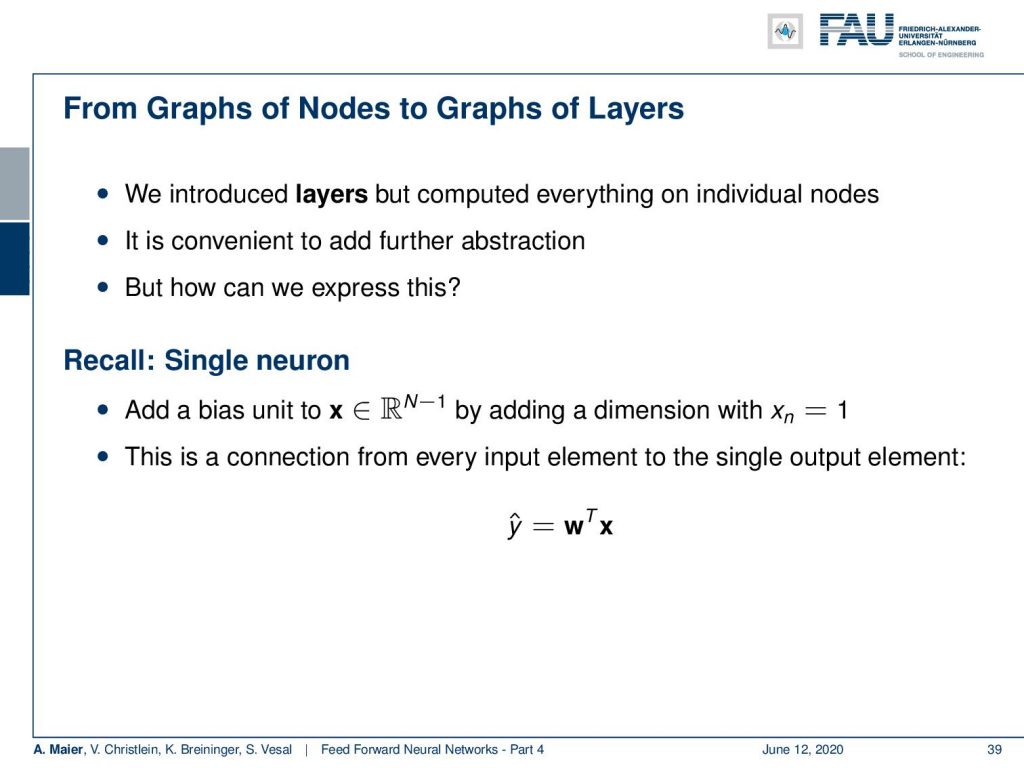
So, how do we express this? Let’s recall what our single neuron is doing. The single neuron is computing essentially an inner product of its weights. By the way, we are skipping over this bias notation. So, we are expanding this vector by one additional element. This allows us to describe the bias also and the inner product as shown on the slide here. This is really nice because then you can see that the output y hat is just an inner product.
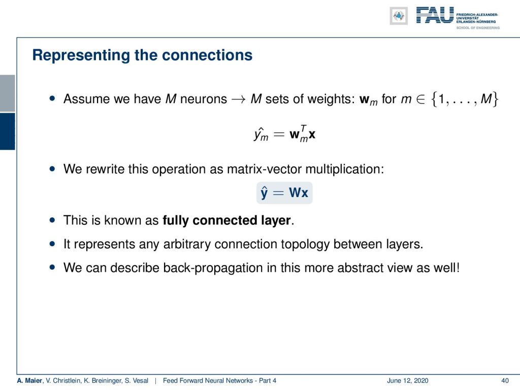
Now think about the case that we have M neurons which means that we get some y hat index m. All of them are inner products. So, if you bring this into a vector notation, you can see that the vector y hat is nothing else than a matrix multiplication of x with this matrix W. You see that a fully connected layer is nothing else than matrix multiplication. So, we can essentially represent arbitrary connections and topologies using this fully connected layer. Then, we also apply a pointwise non-linearity such that we get the nonlinear effect. The nice thing about matrix notation is of course that we can describe now the entire layer derivatives using matrix calculus.
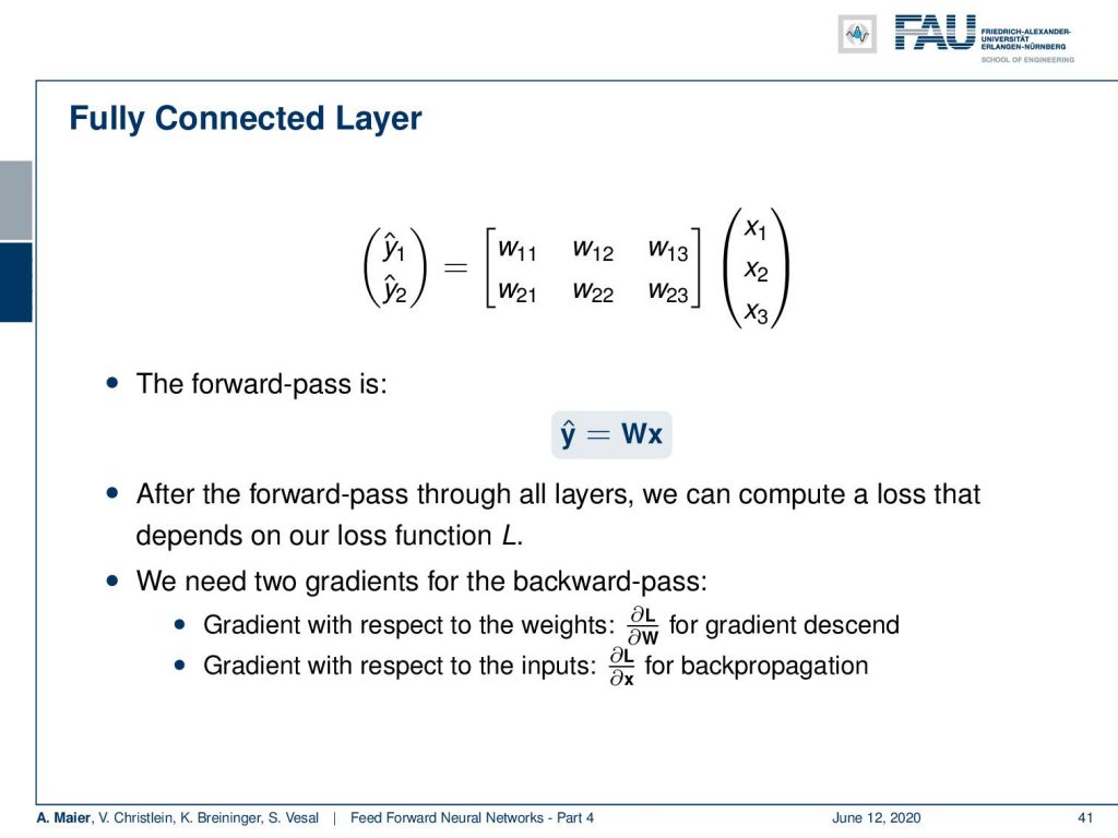
So, our fully connected layer would then get the following configuration: Three elements for the input and then weights for every neuron. Let’s say you have two neurons, then we get these weight vectors. We multiply the two with x. In the forward pass, we have determined this y hat for the entire module using a matrix. If you want to compute the gradients, then we need exactly two partial derivatives. These are the same as we already mentioned: We need the derivative with respect to the weights. This is going to be the partial derivative with respect to W and the partial derivatives with respect to x for the backpropagation to pass it on to the next module.
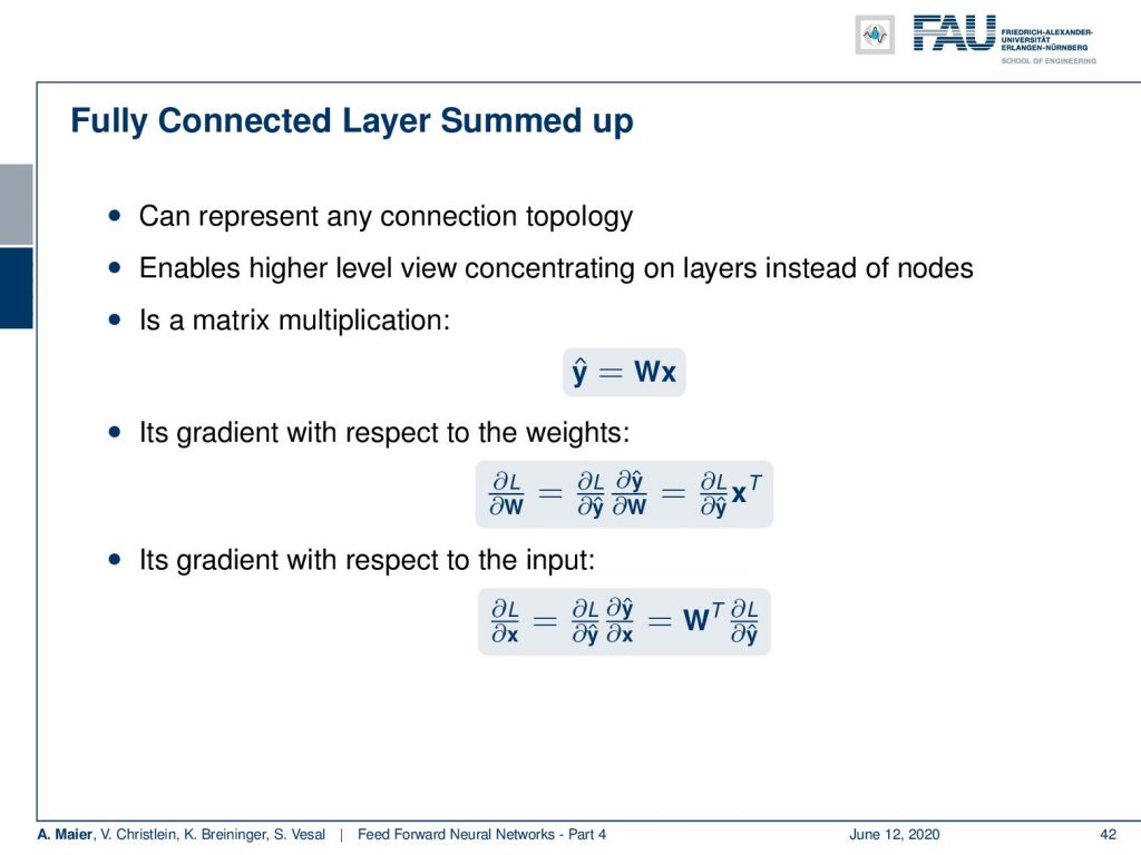
So how do we compute this? Well, we have the layer that is y hat equals to W x. So there’s a matrix multiplication in the forward pass. Then, we need the derivative with respect to the weights. Now you can see that what we essentially need to do is we need a matrix derivative here. The derivative of y hat with respect to W is going to be simply xᵀ. So, if we have the loss that comes into our module, the update to our weights is gonna be this loss vector multiplied with xᵀ. So, we have some loss vector and xᵀ which essentially means that you have an outer product. One is a column vector and the other one is a row vector because of the transpose. So, if you multiply the two, you will end up with a matrix. The above partial derivative with respect to W will always result in a matrix. Then if you look at the bottom row, you need the partial derivative of y hat with respect to x. Also something you can find in the matrix cookbook, by the way. It is very very useful. You find all kinds of matrix derivatives in this one. So if you do that, you can see for the above equation, the partial with respect to x is going to be Wᵀ. Now, you have Wᵀ multiplied again by some loss vector. This loss vector times a matrix is going to be a vector again. This is the vector that you will pass on in the backpropagation process towards the next higher layer.
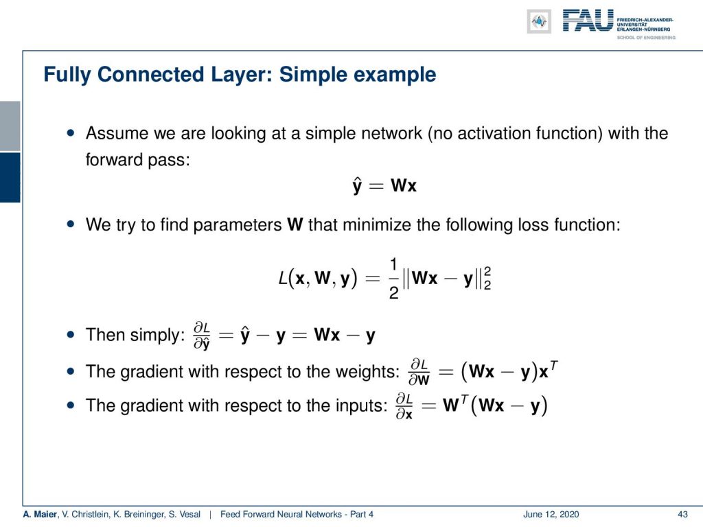
Okay so let’s look into some example. We have a simple example first and then a multi-layer example next. So, the simple example is going to be the same network as we had it already. So this was network without any non-linearity W x. Now, we need some loss function. Here, we don’t take cross-entropy, but we take the L2 loss which is a common vector norm. What it does is simply take the output of the network subtract and the desired output and compute the L2 norm. This means that we element-wise square the different vector values and sum all of them up. In the end, we would have to take a square root, but we want to omit this. So, we take it to the power of two. When we now compute the derivatives of this L2-norm to the power of 2, of course, we have a factor of two showing up. This will be canceled out by this factor 1 over 2 in the beginning. By the way, this is a regression loss and also has statistical relations. We will talk about this when we talk about loss functions in more detail. The nice thing with L2 loss is that that you also find its matrix derivatives the matrix cookbook. We now compute the partial derivative of L with respect to y hat. This will give us then Wx – y and we can continue and compute the update for our weights. So the update for the weights is what we compute using the loss function’s derivative. The derivative of the loss function with respect to the input was Wx – y times xᵀ. This will give us an update for the matrix weight. The other derivative that we want to compute is the partial derivative of the loss with respect to x. So, this is going to be – as we’ve seen on the previous slide – Wᵀ times the vector that comes from the loss function: Wx – y, as we determined in the third row of the slide.
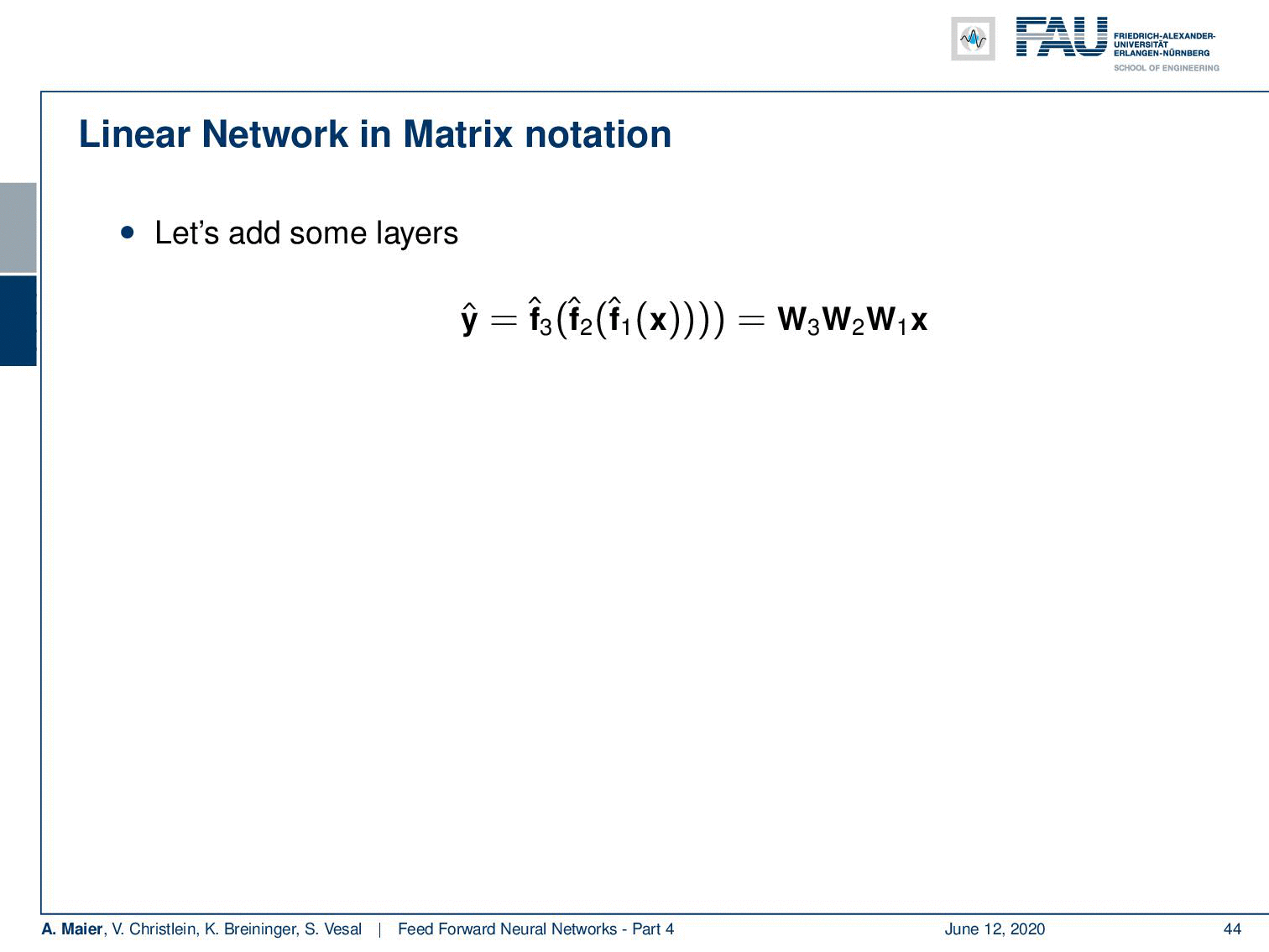
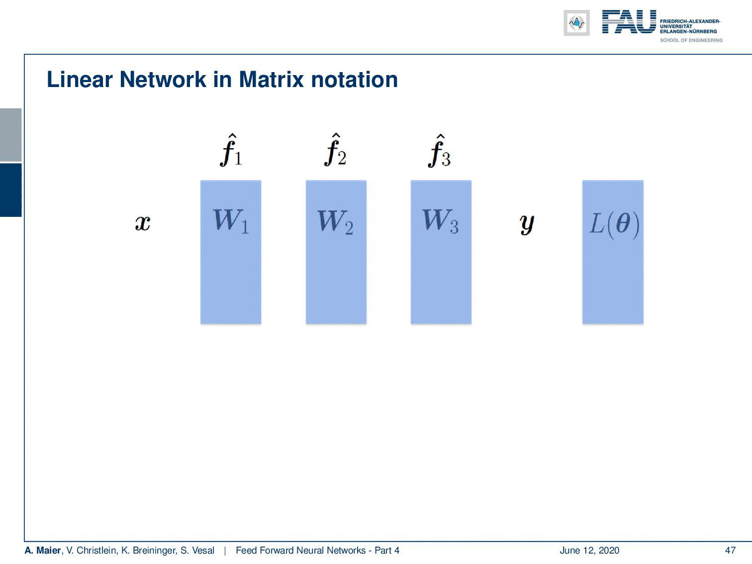
Ok so let’s add some layers and change our estimator into three nested functions. Here, we have some linear matrices. So, this is an academic example: you could see that by multiplying W₁, W₂, and W₃ with each other, they would simply collapse into a single matrix. Still, I find this example useful because it shows you what actually happens in the computation of the backpropagation process and why those specific steps are really useful. So, again we take the L2 loss function. Here, we have our three matrices inside.
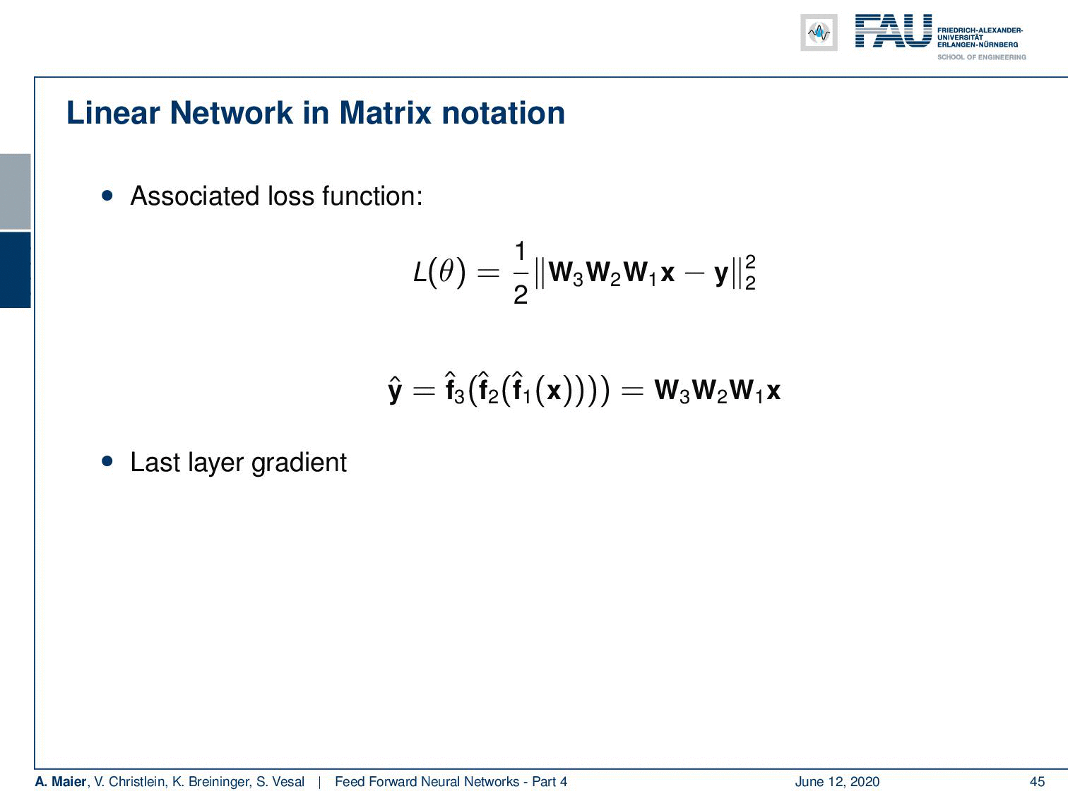
Next, we have to go ahead and compute derivatives. Now for the derivatives, we start with Layer 3, the most outer layer. So, you see that we now compute the partial derivative of the loss function with respect to W₃. First, the chain rule. Then, we have to compute the partial derivative of the loss function with respect to f₃(x) hat with respect to W₃. The partial derivative of the loss function again is simply the inner part of the L2 norm. So is this W₃ W₂ W₁ x – y. The partial derivative of the net is gonna be (W₂ W₁ x)ᵀ, as we’ve seen on the previous slide. Note that I’m indicating the affinity of the matrix operator using a dot. For matrices, it makes a difference whether you multiply them from the left or from the right. Both multiplication directions are different. Hence, I’m indicating that you have to compute this product from the right-hand side. Now let’s do that and we end up with the final update for W₃ that is simply computed from those two expressions.
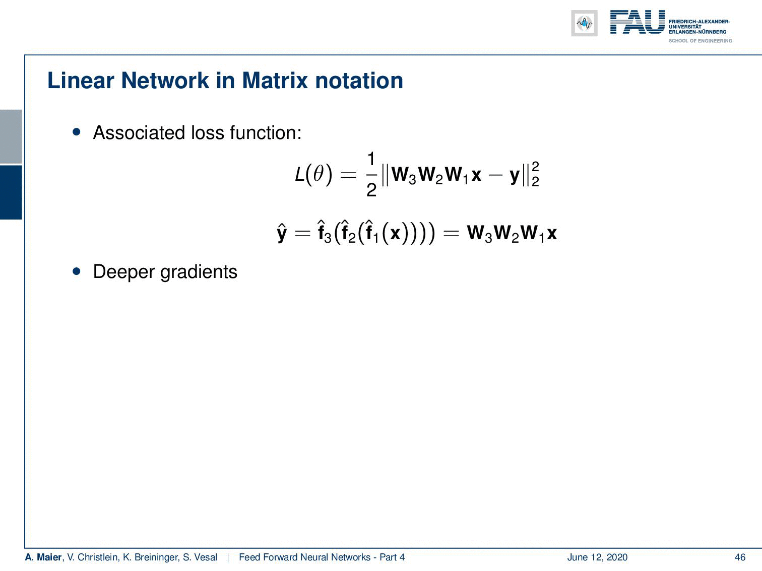
Now, the partial derivative with respect to W₂ is a bit more complicated because we have to apply the chain rule twice. So, again we have to compute the partial derivative of the loss function with respect to f₃(x) hat. Then, we need the partial derivative of f₃(x) hat with respect to W₂ which means we have to apply the chain rule again. So we have to expand the partial derivative of f₃(x) hat with respect to f₂(x) hat and then the partial derivative of f₂(x) hat with respect to W₂. This doesn’t change much. The Loss term is the same as we used before. Now, if we compute the partial derivative of f₃(x) hat with respect to f₂(x) hat – remember f₂(x) = W₂ W₁ x – it’s gonna be W₃ᵀ and we have to multiply it from the left-hand side. Then, we go ahead and compute the partial derivative of f₂(x) hat with respect to W₂. You remain with (W₂ W₁ x)ᵀ. So, the final matrix derivative is going to be the product of the three terms. We can repeat this for the last layer, but now we have to apply the chain rule again. We see already two parts that we pre-computed, but we have to apply it again. So here we then get the partial derivative of f₂(x) hat with respect to f₁(x) hat and a partial derivative of f₁(x) hat with respect to W₁ which then yields two terms that we used before. The partial derivative of f₂(x) hat with respect to f₁(x) hat is W₁ x, is going to be W₂ᵀ. Then, we still have to compute the partial derivative of f₁(x) with respect to W₁. This is going to be xᵀ. So, we end up with the product of four terms for this partial derivative.
Now, you can see if we do the backpropagation algorithm, we end up in a very similar way of processing. So first, we compute the forward path through our entire network and evaluate the loss function. Then, we can look at the different partial derivatives, and depending on where I want to go, I have to compute the respective partials. For the update of the last layer, I have to compute the partial derivative of the loss function and multiply it with the partial derivative of the last layer with respect to the weights. Now, if I go the second last layer, I have to compute the partial derivative with respect to the loss function, the partial derivative of the last layer from respect to the inputs, and the partial derivative of the second last layer with respect to the weights to get the update. If I want to go to the first layer, I have to compute all the respective backpropagation steps for the entire layers until I end up with the respective update on the very first layer. You can see that we can pre-compute a lot of those values and reuse them which allows us to implement backpropagation very efficiently.
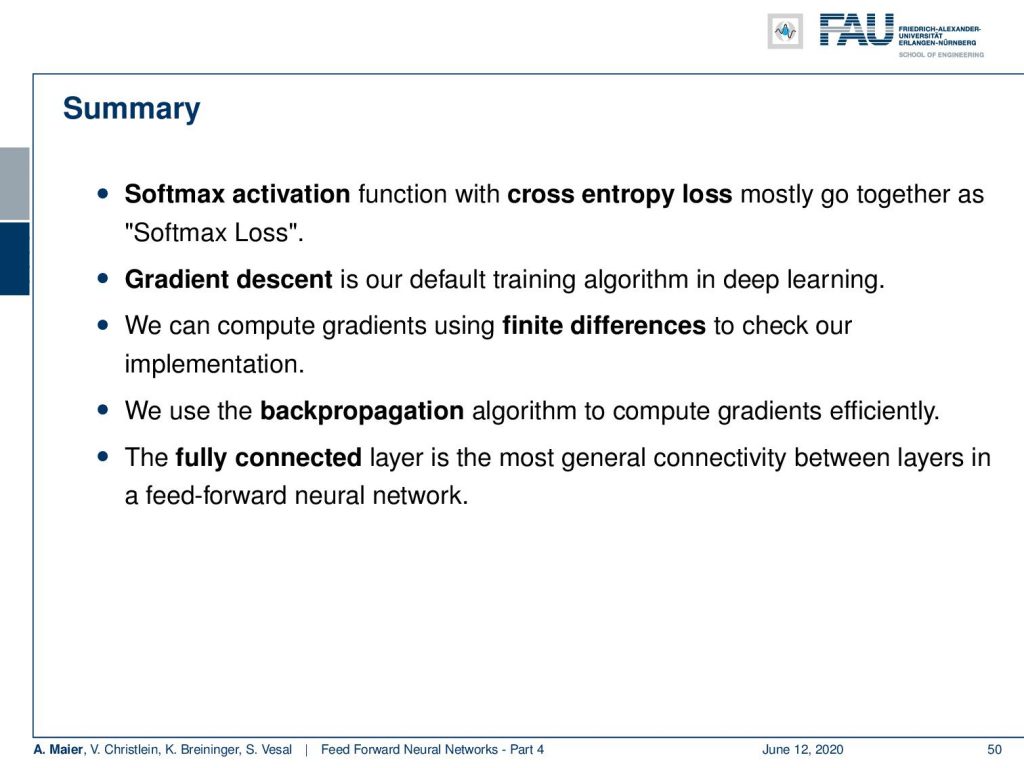
Let’s summarize what we’ve seen so far. We’ve seen that we can combine the softmax activation function with the cross-entropy loss. Then, we can very naturally work with multi-class problems. We used gradient descent as the default choice for training network and we can achieve local minima using the strategy. We can, of course, compute gradients only numerically by finite differences and this is very useful for checking your implementations. This is something you will definitely need in the exercises! Then, we used the backpropagation algorithm to compute the gradients very efficiently. In order to be able to update the weights of the fully connected layers, we’ve seen that they can be abstracted as a complete layer. Hence, we can also compute layer-wise derivatives. So, it’s not required to compute everything on a node level, but you can really go into layer abstraction. You also saw that matrix calculus turns out to be very useful.
What happens next time in deep learning? Well, we will see that right now, we have only a limited number of loss functions. So, we will see problem adapted loss functions for regression and classification. The very simple optimization that we talked about right now with a single η is probably not the right way to go. So, there are much better optimization programs. They can be adapted to the needs of every single parameter. Then we’ll also see an argument why neural networks shouldn’t perform that well and some recent insights why they actually do perform quite well.
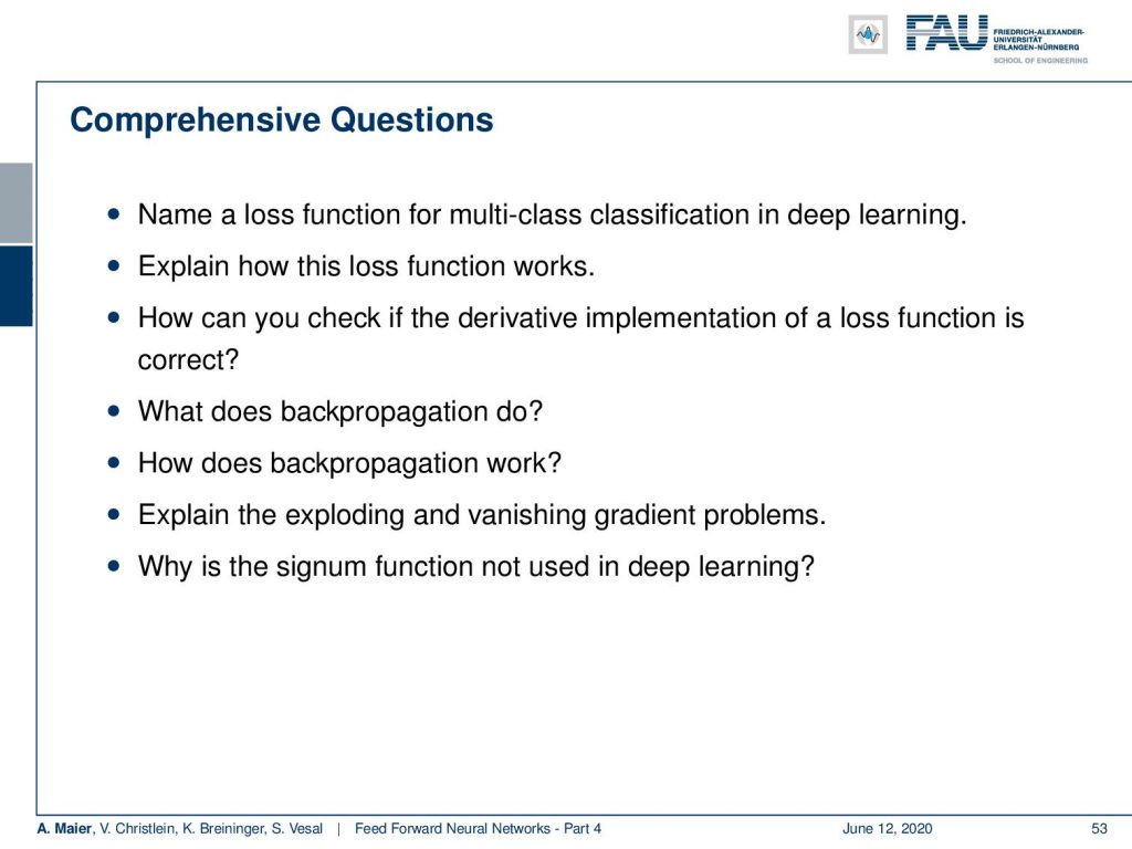
I also have a couple of comprehensive questions. So you should definitely be able to name different loss functions for multi-class classification. One-hot encoding is something everybody needs to know if you want to take the oral exam with me. You will have to be able to describe this. Then, of course, something I probably won’t ask in the exam but something that will be very useful for your daily routine is that you work with finite differences and use them for implementation checks. You have to be able to describe the backpropagation algorithm and to be honest, I think this – although it’s academic – but this multi-layer way abstraction way of describing backpropagation algorithm is really useful. It’s also very nice if you want to explain the backpropagation in an exam situation. What else do you have to be able to describe? The problem with exploding and vanishing gradients: What happens if you choose your η too high or too low? What’s a lost curve and how does it change over the iterations? Take a look at those graphs. They are really relevant and they also help you understand what’s going wrong in your training process. So you need to be aware of those and also it should be clear to you by now why the sign function is a bad choice for an activation function. We have plenty of references below this post. So, I hope you still had fun with those videos. Please continue watching and see you in the next video!
If you liked this post, you can find more essays here, more educational material on Machine Learning here, or have a look at our Deep Learning Lecture. I would also appreciate a clap or a follow on YouTube, Twitter, Facebook, or LinkedIn in case you want to be informed about more essays, videos, and research in the future. This article is released under the Creative Commons 4.0 Attribution License and can be reprinted and modified if referenced.
References
[1] R. O. Duda, P. E. Hart, and D. G. Stork. Pattern Classification. John Wiley and Sons, inc., 2000.
[2] Christopher M. Bishop. Pattern Recognition and Machine Learning (Information Science and Statistics). Secaucus, NJ, USA: Springer-Verlag New York, Inc., 2006.
[3] F. Rosenblatt. “The perceptron: A probabilistic model for information storage and organization in the brain.” In: Psychological Review 65.6 (1958), pp. 386–408.
[4] WS. McCulloch and W. Pitts. “A logical calculus of the ideas immanent in nervous activity.” In: Bulletin of mathematical biophysics 5 (1943), pp. 99–115.
[5] D. E. Rumelhart, G. E. Hinton, and R. J. Williams. “Learning representations by back-propagating errors.” In: Nature 323 (1986), pp. 533–536.
[6] Xavier Glorot, Antoine Bordes, and Yoshua Bengio. “Deep Sparse Rectifier Neural Networks”. In: Proceedings of the Fourteenth International Conference on Artificial Intelligence Vol. 15. 2011, pp. 315–323.
[7] William H. Press, Saul A. Teukolsky, William T. Vetterling, et al. Numerical Recipes 3rd Edition: The Art of Scientific Computing. 3rd ed. New York, NY, USA: Cambridge University Press, 2007.