
Class Imbalance
These are the lecture notes for FAU’s YouTube Lecture “Deep Learning“. This is a full transcript of the lecture video & matching slides. We hope, you enjoy this as much as the videos. Of course, this transcript was created with deep learning techniques largely automatically and only minor manual modifications were performed. If you spot mistakes, please let us know!
Welcome back to deep learning! Today, we want to continue talking about our common practices. The methods that we are interested in today are about class imbalance. So, a very typical problem is that one class – in particular the very interesting one – is not very frequent. So, this is a challenge for all the machine learning algorithms.
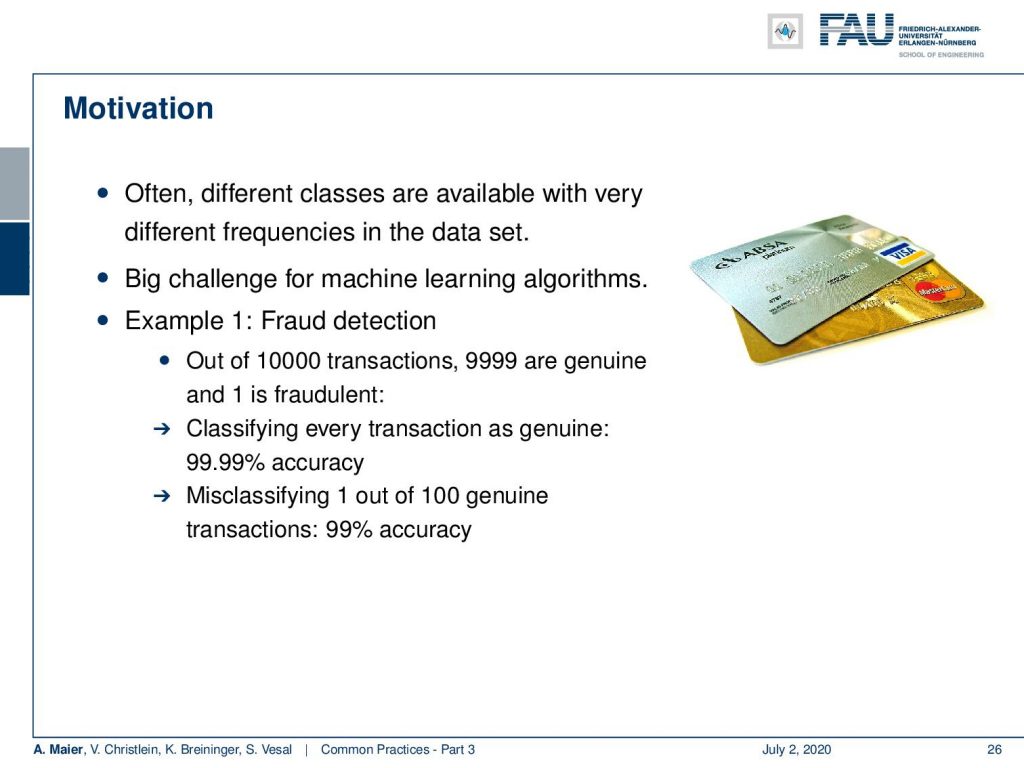
Let’s take the example of fraud detection. Out of 10,000 transactions, 9,999 are genuine and only one is fraudulent. So, if you classify everything as genuine, you get 99.99% accuracy. Obviously, even in less severe situations, we are if you had a model and that would misclassify one out of a hundred transactions, then you would end up only in a model with 99% accuracy. This is of course a very hard problem. In particular, in screening applications, you have to be very careful because just classifying everything to the most common class would still get you very very good accuracy.
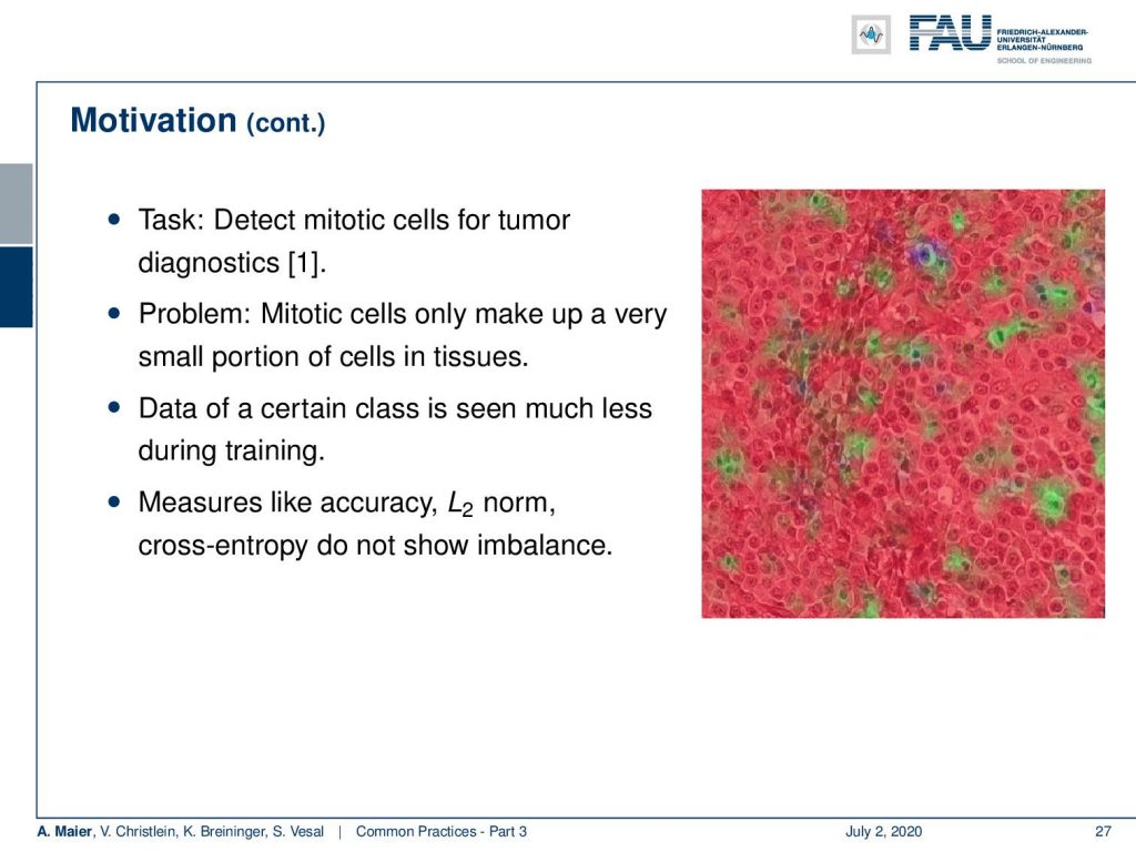
It doesn’t have to be credit cards, for example, here detecting mitotic cells is a very similar problem. A mitotic cell is a cell undergoing cell division. These cells are very important as we already heard in the introduction. If you count the cells under mitosis, you know how aggressively the associated cancer is growing. So this is a very important feature but you have to detect them correctly. They make up only a very small portion of the cells in tissues. So, the data of this class has been seen much less during the training, and measures like the accuracy, L2 norm, and cross-entropy don’t show this imbalance. So, they are not very responsive to this.
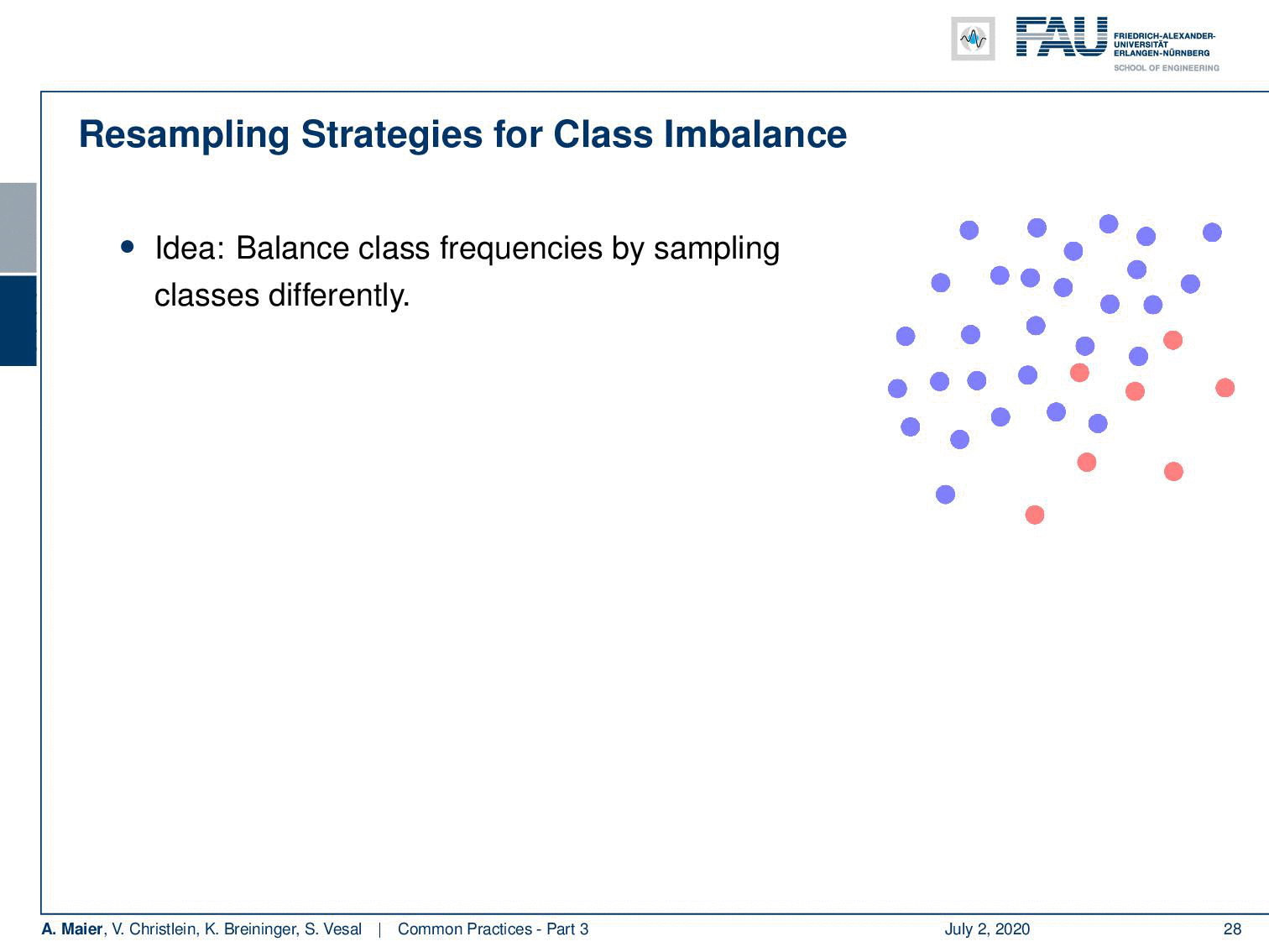
One thing that you can do is for example resampling. The idea is that you balance the class frequencies by sampling classes differently, So, you can understand this means that you have to throw away a lot of the training data of the most frequent classes. This way you get to train a classifier that will be balanced towards both of these classes. Now they are seen approximately as frequently as the other class. The disadvantage of this approach is that you’re not using all the data that is being seen and of course, you don’t want to throw away data.
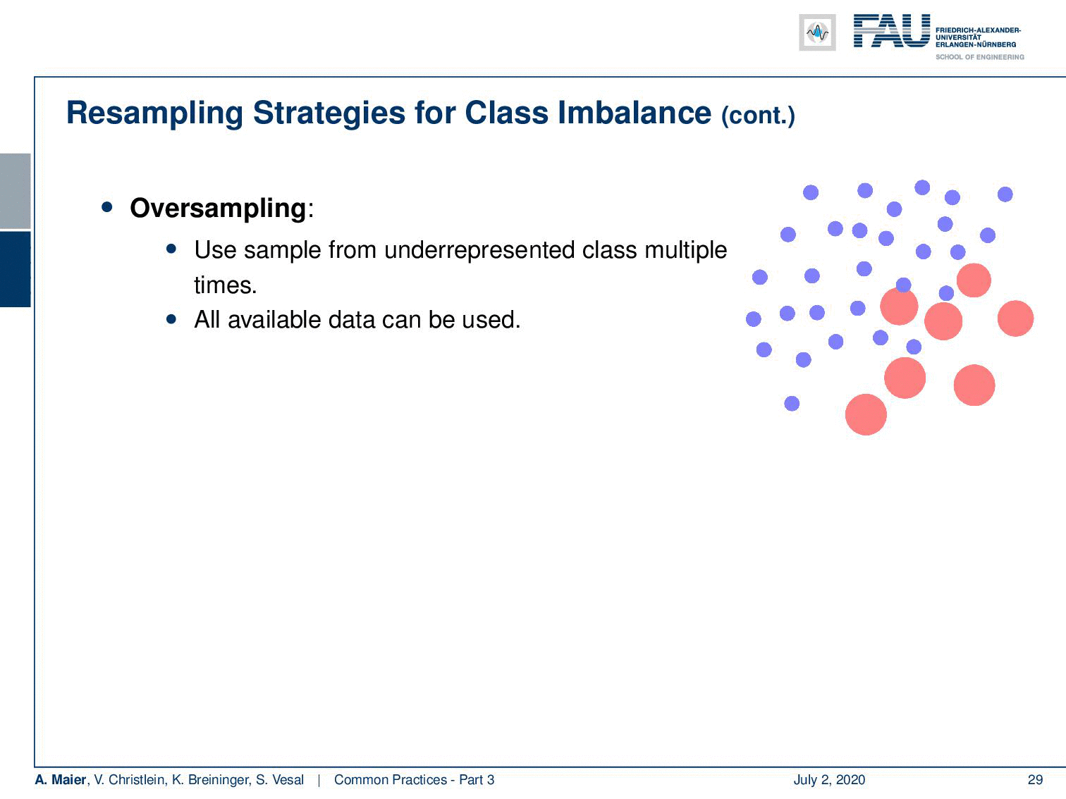
So another technique is oversampling. You can just sample more often from the underrepresented classes. In this case, you can use all of the data. The disadvantage is of course that it can lead to heavy overfitting towards the less frequently seen examples. Also possible are combinations of under and oversampling.
This then leads to advanced resampling techniques that try to avoid the shortcomings of undersampling by a synthetic minority oversampling. It’s rather uncommon in deep learning. Underfitting caused by undersampling can be reduced by taking a different subset after each epoch. This is quite common and also you can use data augmentation to help reducing overfitting for underrepresented classes. So, you essentially augment more of the samples that you have seen less frequently.
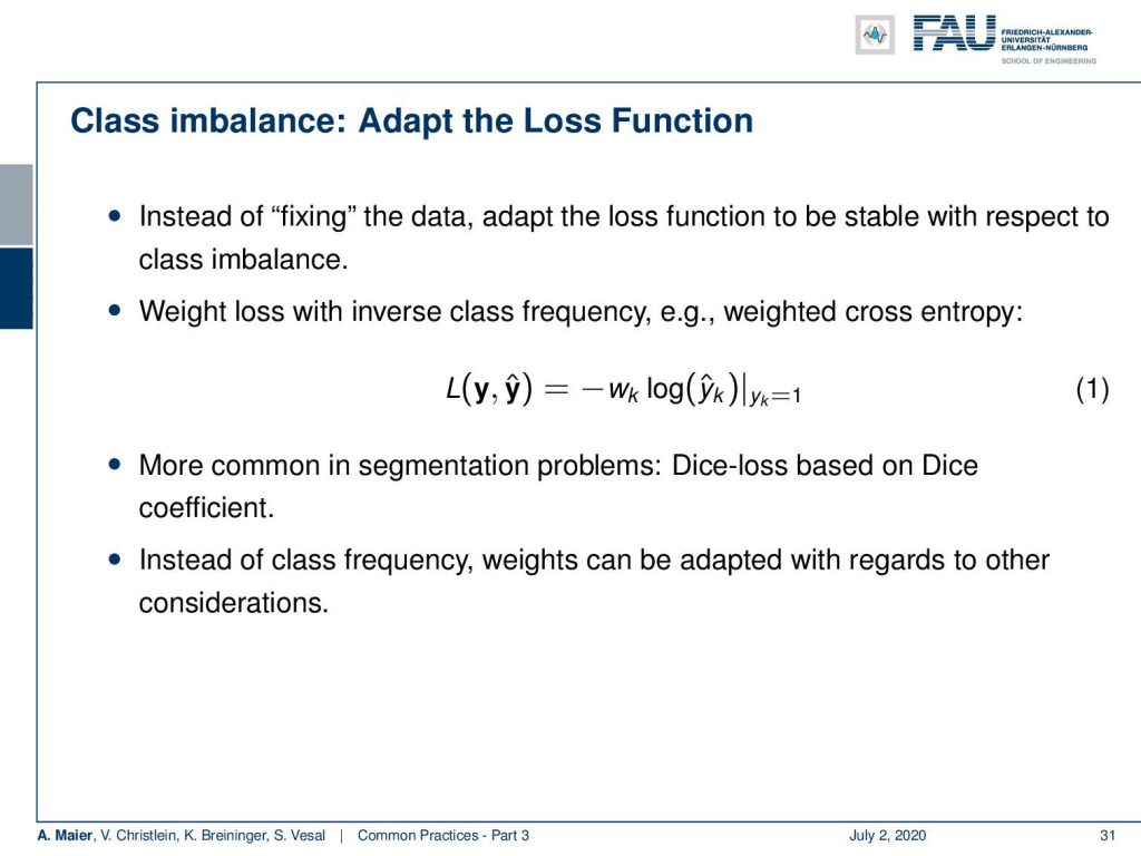
Instead of fixing the data, of course, you can also try to adapt the loss function to be stable with respect to class imbalance. Here, you then choose a loss with the inverse class frequency. You can then create the weighted cross entropy where you introduce an additional weight w which is simply determined as the inverse class frequency. More common in segmentation problems are then things like the Dice loss based on the Dice coefficient. Here, you evaluate the loss on the dice coefficient that measures area overlap. It is a very typical measure for evaluating segmentations instead of class frequency. Weights can also be adapted with regards to other considerations but we are not discussing them here in this current lecture.
This already brings us to the end of this part and in the final section of common practices, we will now discuss measures of evaluation and how to evaluate our models appropriately. So, thank you very much for listening and goodbye!
If you liked this post, you can find more essays here, more educational material on Machine Learning here, or have a look at our Deep LearningLecture. I would also appreciate a follow on YouTube, Twitter, Facebook, or LinkedIn in case you want to be informed about more essays, videos, and research in the future. This article is released under the Creative Commons 4.0 Attribution License and can be reprinted and modified if referenced.
References
[1] M. Aubreville, M. Krappmann, C. Bertram, et al. “A Guided Spatial Transformer Network for Histology Cell Differentiation”. In: ArXiv e-prints (July 2017). arXiv: 1707.08525 [cs.CV].
[2] James Bergstra and Yoshua Bengio. “Random Search for Hyper-parameter Optimization”. In: J. Mach. Learn. Res. 13 (Feb. 2012), pp. 281–305.
[3] Jean Dickinson Gibbons and Subhabrata Chakraborti. “Nonparametric statistical inference”. In: International encyclopedia of statistical science. Springer, 2011, pp. 977–979.
[4] Yoshua Bengio. “Practical recommendations for gradient-based training of deep architectures”. In: Neural networks: Tricks of the trade. Springer, 2012, pp. 437–478.
[5] Chiyuan Zhang, Samy Bengio, Moritz Hardt, et al. “Understanding deep learning requires rethinking generalization”. In: arXiv preprint arXiv:1611.03530 (2016).
[6] Boris T Polyak and Anatoli B Juditsky. “Acceleration of stochastic approximation by averaging”. In: SIAM Journal on Control and Optimization 30.4 (1992), pp. 838–855.
[7] Prajit Ramachandran, Barret Zoph, and Quoc V. Le. “Searching for Activation Functions”. In: CoRR abs/1710.05941 (2017). arXiv: 1710.05941.
[8] Stefan Steidl, Michael Levit, Anton Batliner, et al. “Of All Things the Measure is Man: Automatic Classification of Emotions and Inter-labeler Consistency”. In: Proc. of ICASSP. IEEE – Institute of Electrical and Electronics Engineers, Mar. 2005.