Lecture Notes in Pattern Recognition: Episode 23 – Support Vector Machines – Concept
These are the lecture notes for FAU’s YouTube Lecture “Pattern Recognition“. This is a full transcript of the lecture video & matching slides. We hope, you enjoy this as much as the videos. Of course, this transcript was created with deep learning techniques largely automatically and only minor manual modifications were performed. Try it yourself! If you spot mistakes, please let us know!
Welcome back to Pattern Recognition. Today we want to start talking about support vector machines. Support vector machines are a very powerful classification technique that is built on top of convex optimization. So you will see that it essentially builds on top of everything that we’ve seen so far in this class. We will see that we can solve some of the problems much more elegantly using the tricks that we will show you in the next couple of videos.
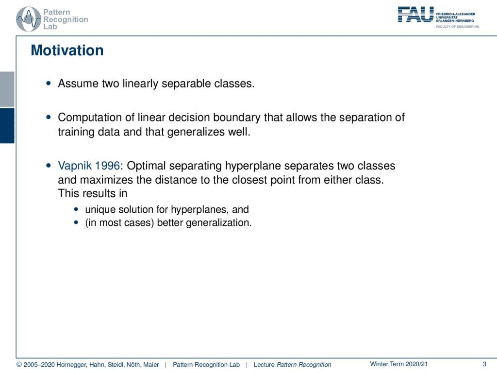
What is our motivation? Well again we want to look into linear decision boundaries and we assume that we have two linearly separable classes. Then we want to compute a linear decision boundary that allows the separation of the training data and that generalizes very well. This builds on some observations by Vapnik and already in 1996, he could show that the optimal separating hyperplane separates two classes and maximizes the distance to the closest point from either class. This then results in a unique solution for the hyperplanes and in most cases better generalization.
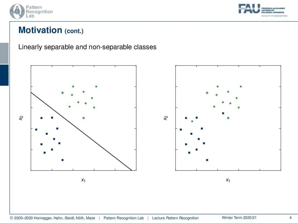
So let’s look into the type of problem that we want to solve. Here we have linearly separable and non-separable cases. On the left-hand side, you can see we have the green and the blue dots and they can be separated with just a single line. So this is a separable case. On the right-hand side, you see a non-separable case. So you see that there are only two points that have been switched and with these two points the problem suddenly becomes no longer solvable with a single hyperplane that would separate the two clusters. So if you remember the perceptron in the right-hand case it would essentially iterate until infinity. Let’s stick first with the separable case on the left-hand side.
Now the problem here is you see that there is quite some space between the two point clouds. This means that there are quite a few different solutions that you can find. Therefore we don’t have a unique solution just by aiming at separating the two classes. So one thing that we could do in this case is for example to average the perceptron solutions. Now the idea that was introduced by Vapnik is actually that you want to maximize the distance between the points of the two classes. Here we actually show a solution that is showing a hyperplane.
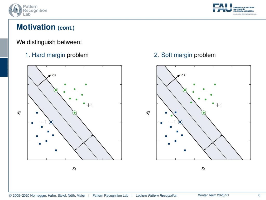
So here you see this line with the normal vector α and this one is essentially maximizing the distance between the two-point sets. So on the left-hand side, we have the hard margin problem. In the hard margin problem, we really require the two sets to be absolutely separable. Then there is the soft margin problem and then the soft margin problem we will use a couple of more tricks to actually also allow then a misclassification. So here you can see that there is one point that cannot be separated in the second point cloud and here we can then introduce tricks in order to still be able to compute a unique decision boundary. This is then called the soft margin problem because we allow some confusions that are caused by the optimally separating hyperplane.
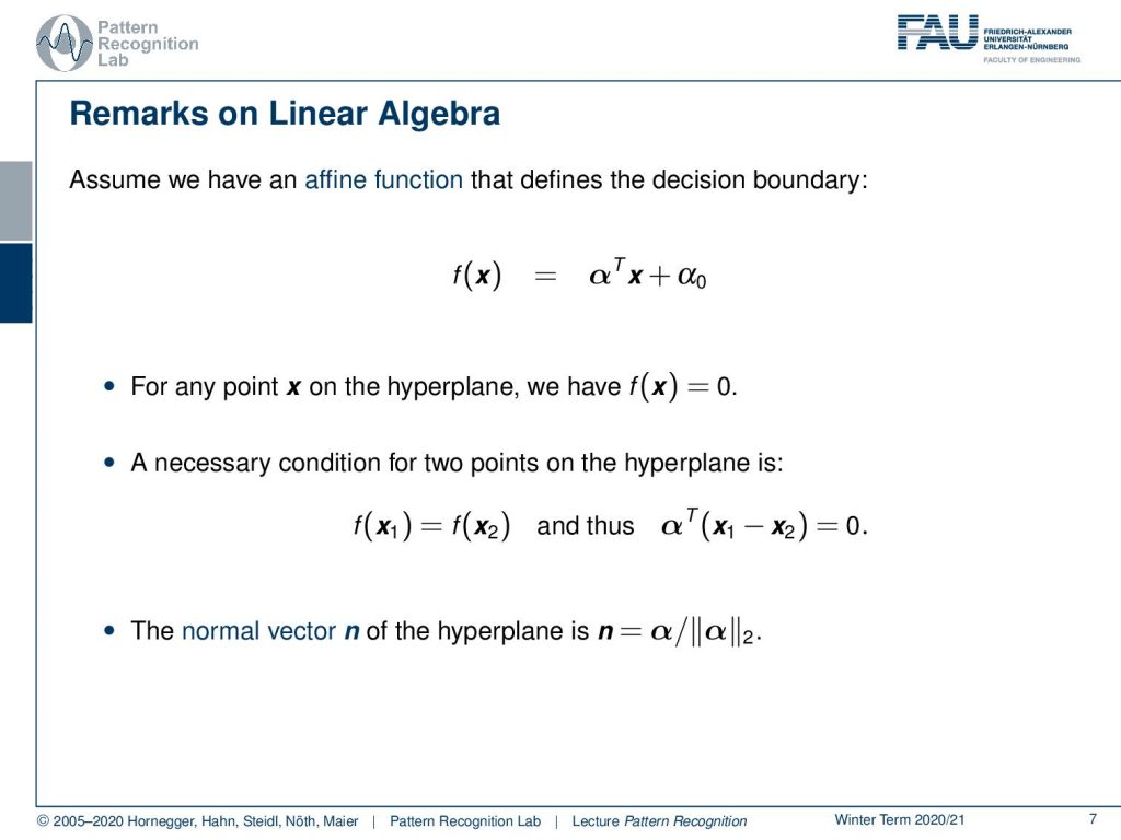
Let’s have a look at a bit of linear algebra. We assume that we have an affine function that defines the decision boundary. So we can write this up simply as the normal vector αTx plus some bias α0. This then means that for any point x on the hyperplane we essentially have f(x) equals to zero. So if you’re on the plane then you have this inner product plus α0 and you will exactly equal to zero. Also if you have two points that are on the hyperplane then the following conditions have to hold: if you have x1 minus x2 and multiply them with αT then also they need to be zero. So this is also a necessary condition for all points x1, x2 that is on the hyperplane. Also, note that the actual normal vector of the hyperplane needs to be normalized with the length. So α is of course a vector that points in the normal vector direction but actually the normal vector you would have to divide by the length of α. So here we take the two norm.
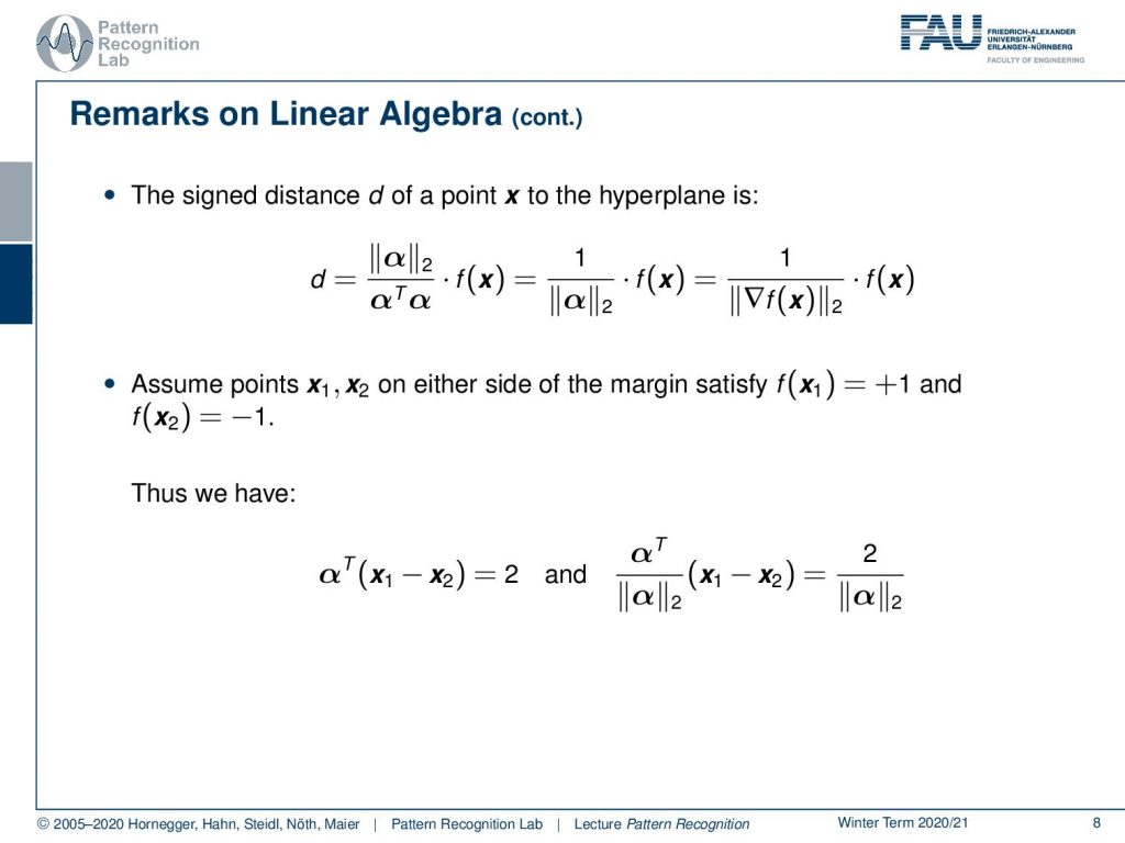
Note that this is very important in particular if you’re considering signed distances. So if you really want to compute signed distances to the hyperplane then actually what you would need to do is you have to scale with the normal vector to compute d that is the signed distance and here you can see different versions of how to write this. But it is essentially f(x) divided by the norm of α and note that if you’re actually computing the gradient of f(x) you will see that the gradient is simply α. So you essentially have a scaled version of f(x) with the magnitude of the gradient. Now then this has some implications regarding the distance. So let’s assume again our two points and let’s say they are actually on the margin. Now the margin is essentially the space that is still available. So these are the two closest points and we can essentially then find the length of the normal vector in a way that it will be exactly one. So if we have two points with this optimally separating hyperplane then αT times x1 minus x2 is exactly 2 because they’re from opposite classes. So they’re from f(x1) is plus 1 and f(x2) is -1, so the distance of the 2 is exactly 2. Now if you want to convert this into a signed distance then you see that you actually have to scale this. In the sign distance case you actually have αT over α norm and then we can compute this as 2 divided by the norm of α. So keep that in mind all the distances are dependent on the norm of α because this gives us really the signed distances.
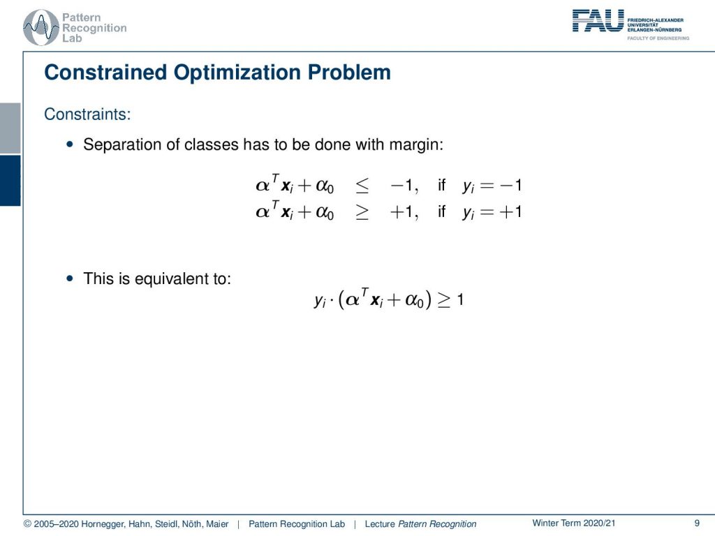
Now let’s look at another property of our system here. The separation of the two classes has to be done with margin meaning that if I compute the distance to this hyperplane then I can essentially compute αTxi plus α0. If it’s in the negative class it needs to be below -1 because we want to keep the margin free. So we want to have a space of one on either side of the decision boundary and therefore also on the other side, we have this relationship that αTxi plus α0 has to be larger than 1 in case we are in the positive class. We can write this up very elegantly and you’ve seen this relation earlier in this class as yi times αTxi plus α0 needs to be greater or equal to 1. So we can take the two inequalities above and write them up in the single one by simply multiplying with the right factor of yi.
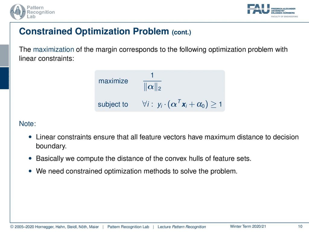
Now we can actually put that into a constrained optimization problem. So here then the maximization of the margin corresponds to the actual maximization of one over the norm of α. Then we have a constraint and actually, we have one constraint for every data point and the constraint is that the data point needs to be on the right side of the decision boundary given the margin of 1. So all features should have a maximum distance to the decision boundary. We essentially compute the distance of the convex hull of the feature sets in this kind of optimization problem. We further need constrained optimization methods to solve the problem because we have the implications on the norm of α and we also need to make sure that all points are projected to the right side.
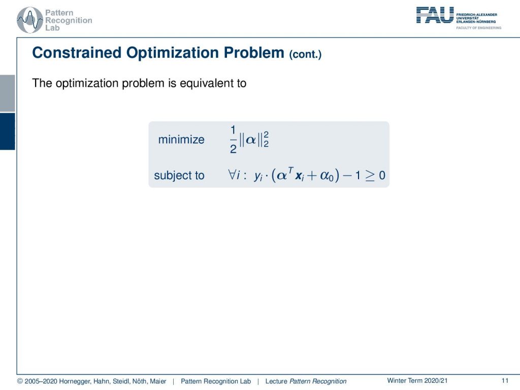
Now let’s rewrite this a little bit in particular the one over α norm is not so great and also the constraints we can still essentially subtract -1 and put them in inequality constraints that are greater to zero. So if I do that our maximization turns into a minimization because I simply flip the fraction and I add and 1 over 2 such that we also then have nicer derivatives. So if you take the derivative of the square two norm then the one over two will cancel out so we still have this nice property that the derivative of this function is simply going to be α. Now we also need the constraints and you see that I simply subtracted minus 1 in order to bring this into inequality constraints regarding zero.
Some remarks on this optimization problem it’s a convex optimization problem. There exist efficient algorithms for solving this problem for example the interior point method and standard libraries for constrained minimization support the solution. Also, the solution is unique.
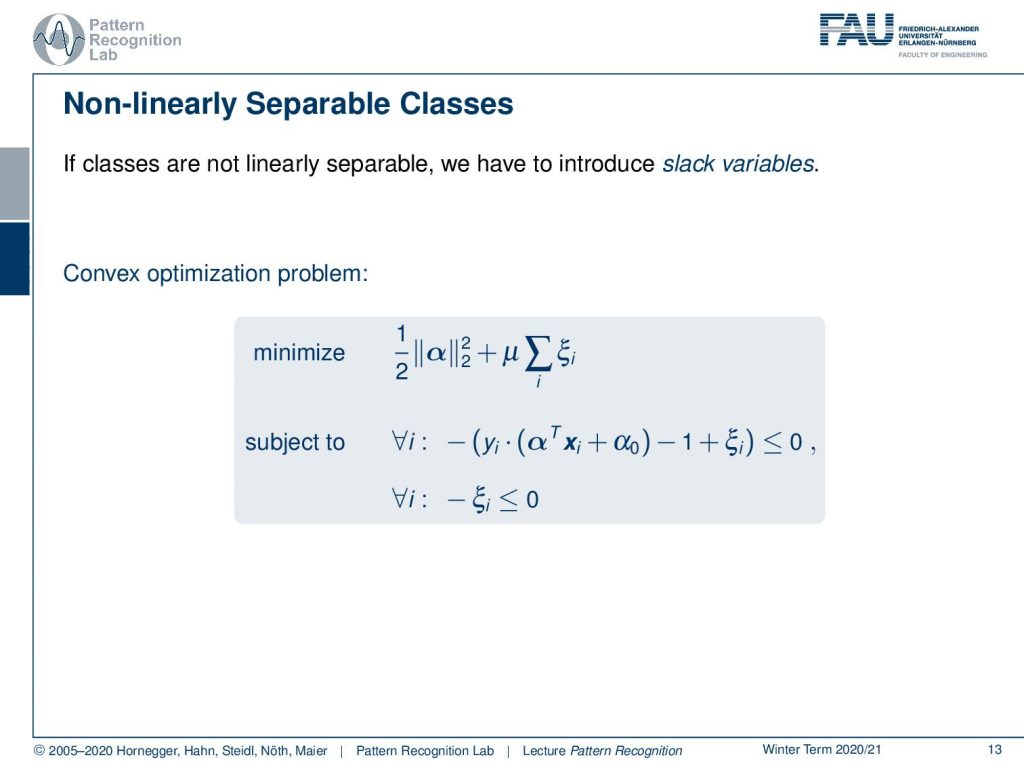
Let’s look a bit into the non-linearly separable classes so if the classes are not linearly separable we have to introduce something that is called slack variables. The slack variables are introduced here as ξi. It is essentially a small value that we can add on top. So let’s say our constraint is not fulfilled and we are on the wrong side of the decision boundary. Then we can give some slack and we just add a small value just to move it to the right side of the decision boundary. Of course, we don’t want to do that for all our points. This is why we include the sum over all ξi into the minimization problem. So we want the size to be small. So only very few points should be altered by our slack variables and then we have essentially again a convex optimization problem where we have the norm of α and then in addition μ times the sum over all the ξis. We have again the inequality constraints note they are now extended with ξi to give the slag for sorting out misclassifications. Then we also have the constraint that minus ξi needs to be negative for all our ξi which we also need to embed into the optimization. So this is then the idea of how we can tackle the cases where the classes are not linearly separable such that we can still apply our support vector machines. So we are not doomed in the case that we are not able to separate all of the points. This can be dealt with with the slack variables.
So what are the lessons that we learned in this small video? We introduced the support vector machine. We introduced the general idea of maximizing the margin between the two classes. We introduced the optimization problems in particular the hard and the soft margin problem. We’ve seen that this is a convex optimization problem. Now actually it’s a strong convex optimization problem which means that there is something that is really fancy the so-called concept of duality holds here.

This is something that we talked about in the next video. So there we actually introduce strong convexity and also the concept of duality.
I do have some further readings for you in particular the works by Schölkopf and Smola. They have been forming this entire field of support vector machines and they have this wonderful book of Learning with Kernels that I can definitely recommend. There’s also the Nature of Statistical Learning Theory by Vapnik which is also a very good recommendation for you. Again Stephen Boyd and Vandenberghe Convex Optimization we will use quite a bit of this in the next couple of videos as well.
So I also have prepared some comprehensive questions. I hope you liked this little video and I’m looking forward to seeing you in the next one. Thank you very much and bye-bye!
If you liked this post, you can find more essays here, more educational material on Machine Learning here, or have a look at our Deep Learning Lecture. I would also appreciate a follow on YouTube, Twitter, Facebook, or LinkedIn in case you want to be informed about more essays, videos, and research in the future. This article is released under the Creative Commons 4.0 Attribution License and can be reprinted and modified if referenced. If you are interested in generating transcripts from video lectures try AutoBlog
References
- Bernhard Schölkopf, Alexander J. Smola: Learning with Kernels, The MIT Press, Cambridge, 2003.
- Vladimir N. Vapnik: The Nature of Statistical Learning Theory, Information Science and Statistics, Springer, Heidelberg, 2000.
- S. Boyd, L. Vandenberghe: Convex Optimization, Cambridge University Press, 2004. ☞http://www.stanford.edu/~boyd/cvxbook/