Lecture Notes in Pattern Recognition: Episode 39 – The Viola-Jones Algorithm

These are the lecture notes for FAU’s YouTube Lecture “Pattern Recognition“. This is a full transcript of the lecture video & matching slides. We hope, you enjoy this as much as the videos. Of course, this transcript was created with deep learning techniques largely automatically and only minor manual modifications were performed. Try it yourself! If you spot mistakes, please let us know!
Welcome back to Pattern Recognition. Today we want to have the last video of our lecture and we actually want to look into an application of Adaboost and this is going to be the Viola-Jones algorithm that was published in 2001.
So the Viola-Jones algorithm is really famous because it solved the face detection problem. It’s using integral images for the feature computation and it uses Adaboost for the actual classification. Then this is building a classifier cascade for the fast rejection of non-phase regions. Various implementations are available. For example: in OpenCV, the phase detector sample is actually implementing Adaboost.
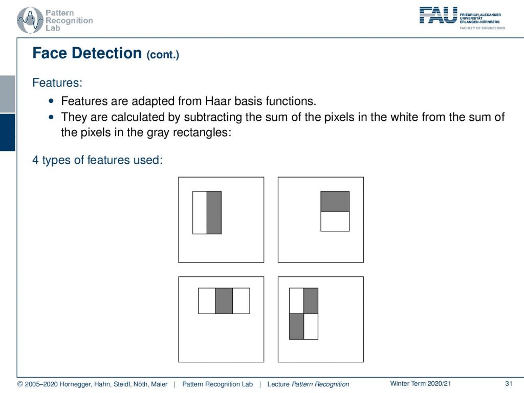
So how do the features work? Well, they are built from a har basis functions. If you attended the introduction to pattern recognition you will know them already. Then you calculate them by subtracting essentially the sum of the pixels in the white from the sum of the pixels in the gray rectangles. There are four different kinds of features that are used: left-right, top-bottom, then center with the sides, and this kind of checkerboard patch.
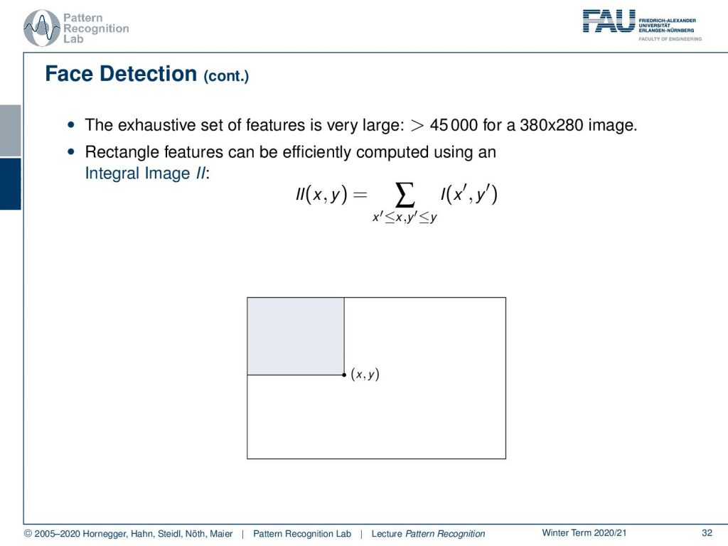
Now in order to do that very quickly the set of features is really large. So if you look at this you have more than 45000 features for a 380×280 image. So the rectangle features need to be computed very efficiently. This is done using integral images and the integral image here indicated by II is essentially returning the integral over the rectangle to the top left. Now if you want to compute arbitrary integrals within the original image from the integral image, you can use the following trick:
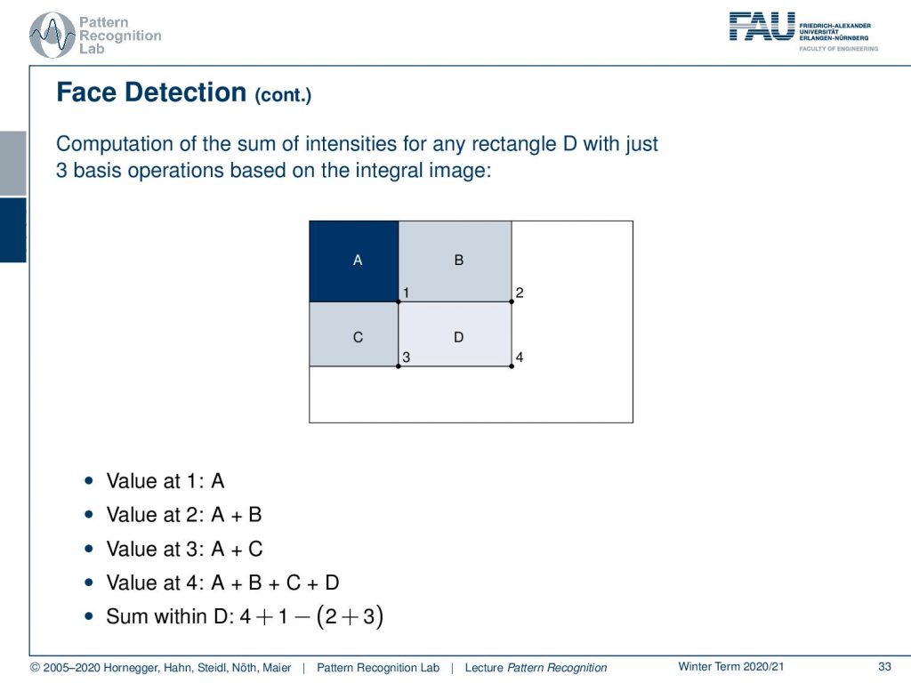
So we have four regions here. A, B, C, and D and we have then values from the integral image. So the value at one is exactly the integral over A. The value of 2 is the integral over A plus B. The value at 3 is the integral over A plus C and the value at 4 is the integral over A plus B plus C plus D. This essentially means that you can compute the integral in D as four plus one minus two plus three. So you essentially subtract A here two times. This is why you need to add it back once in order to compute this integral of D very quickly. So you can compute any rectangular integral in the original image just using the addition and subtraction of four values from the integral image.
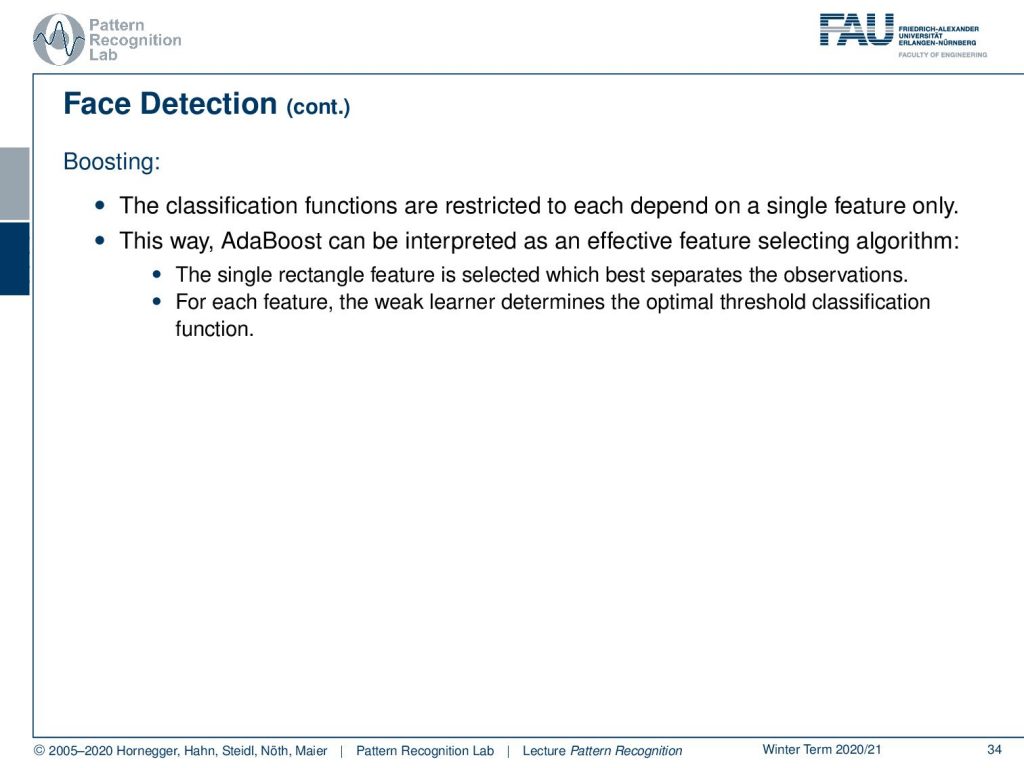
Now they also apply boosting. So the classification functions are restricted to depend on a single feature only. Then this way you can essentially say that Adaboosts can be interpreted as an effective feature selection algorithm. So the single rectangle feature is selected which best separates the observations for each feature the weak learner then determines the optimal threshold classification function.
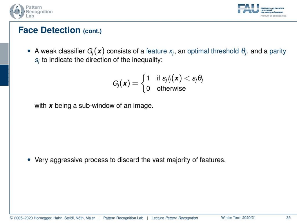
A weaker classifier then consists of a feature Xj and an optimal threshold θj and a parity Sj to indicate the direction of the inequality. So we have very simple classifiers here which is essentially just evaluating the threshold and the parity and here x is being a sub-window of an image. So this is a very aggressive process to discard the vast majority of features and it allows you to build such a boosting cascade.
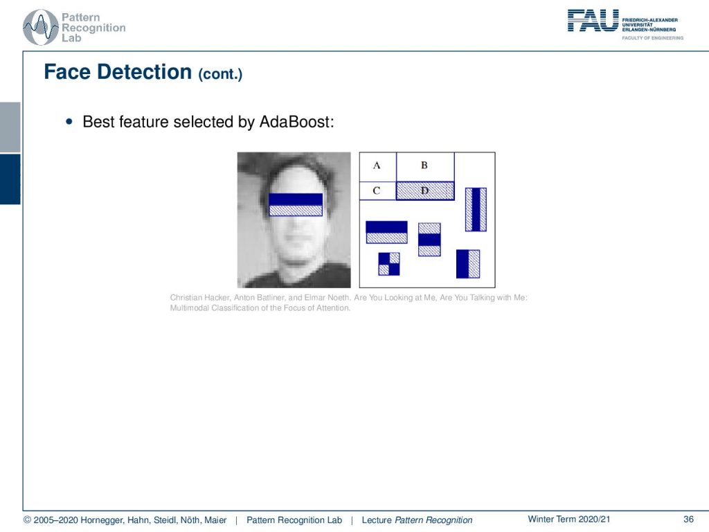
Interestingly you can then have a look at the best features selected here by AdaBoost and this is work by my colleague Christian Hacker. You see that the one feature that is selected virtually always is a patch over the eyes and the nose. You just subtract the two integral images and this is a very very good predictor already for faces. Then of course you need some additional classifications in order to really make sure that these are faces. But this is the best feature that is selected by AdaBoost. So that’s very interesting that we also have this nice interpretation here.
Now we built this classifier cascade and this then means that we have to evaluate a different feature in every step of this boosting process and as soon as we have a misclassification, so it’s not a phase we just stop following that particular position and this allows us to classify really quickly. So you don’t want to evaluate the full AdaBoost sequence on all sub-windows of the image and you just board after you find a negative example. So this simple classify is used to reject the majority of sub-windows and when you build this each stage is created again by AdaBoost. Stage one is essentially using the two features as shown before and detects 100% of the faces with a false positive rate of around 40 percent.
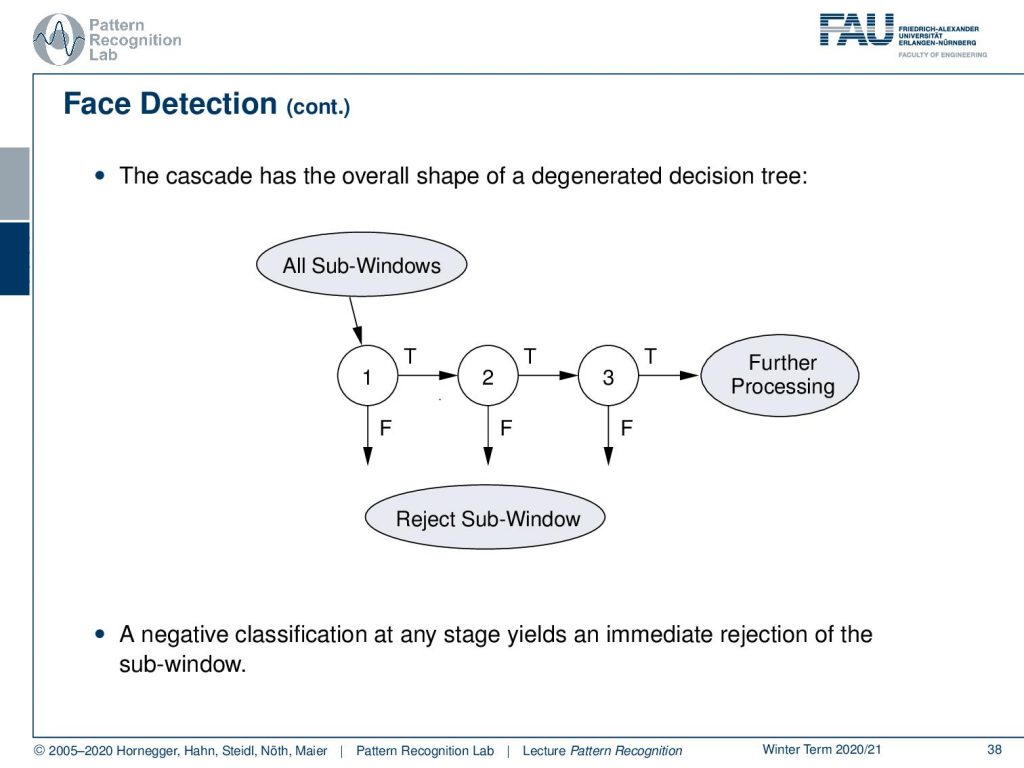
So then the procedure goes like this. So you have all possible sub-windows and then you reject in the first classifier already quite a few of them. Then in the second classifier, you reject more class sub-windows and you follow this cascade over the different steps until you have then a limited number of possible phase candidates that you then actually want to show. So a negative classification at any stage yields an immediate rejection of the sub-window and thereby saves compute time. So the algorithm is very very efficient so that at later points this algorithm is also used on embedded devices on smartphones, on cameras, and so on. So it’s a super-efficient method.
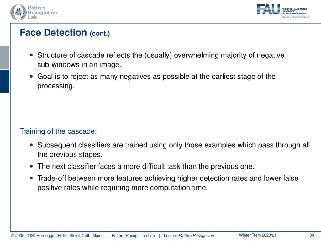
The structure of the cascade reflects usually the overwhelming majority of negative supplements in an image. Now the goal is to reject as many negatives as possible at the earliest stage of processing. Now the training of the cascade is done in subsequent classifiers using only those samples which pass through all of the previous stages. The next classifier then faces a more difficult task than the previous one and of course, there is a train off between more features achieving higher detection rates and lower false-positive rates while requiring more computation time.
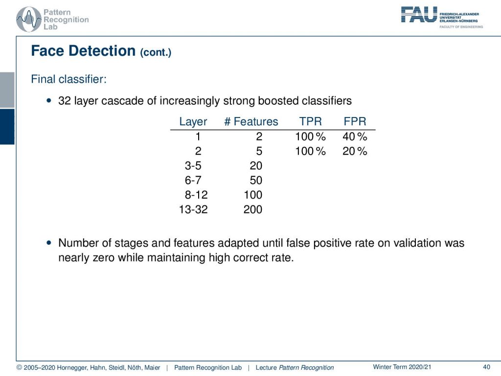
So in the final classifier that we want to demonstrate here, we have a 32 layer cascade of an increasingly strong boosted classifier. In layer one, you only have two features and in layer two you have five features and then gradually the number of features is increasing because you have fewer samples that you actually have to process. So you can spend more time there. So the number of stages and features is adapted until the false positive rate on validation data was nearly zero while maintaining a high correct rate.
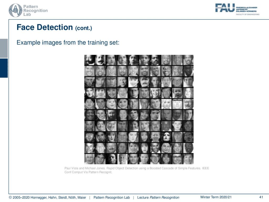
Here you can see example images from the training set. So you see there is huge variability. So it’s also a very big training data set and this was also then used on as said embedded devices.
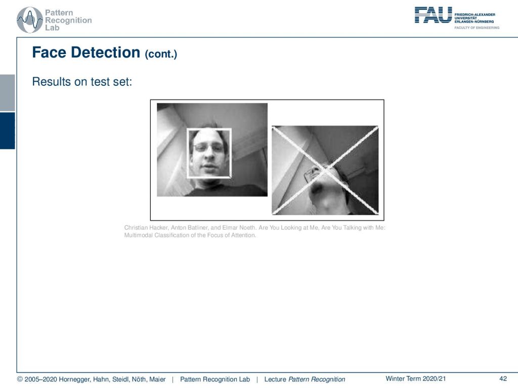
So here you can example see a smartphone recognizing the user whether he is actually looking at the camera or looking away from the camera. This is actually a result of the research project Smartweb.
So what are the lessons that we learned here boosting of weak classifiers can yield powerful combined classifiers? By the way boosting also turned out to be very successful over the years. The famous Netflix challenge was finally also solved with an ensemble technique like boosting. So we introduced the AdaBoost algorithm and looked also into its mathematical details linking it to the exponential loss function. We’ve seen that the weights of the classifier and the data are adjusted during the training. We see that this kind of classification system was put into use in Viola and John’s face detection algorithm.
Of course, I have some further reading for you. Again the Elements of Statistical Learning, then the general paper to boosting and of course Viola and Jones contribution in the international journal of computer vision for robust real-time face detection which was an extremely popular method and has been applied in many many systems in order to detect faces. Also, there is a wonderful introduction to the AdaBoost algorithm that has been created by the technical university in Prague by the center for machine perception. So I hope you enjoyed this small lecture series. This is already the end of our lecture and I think you got now a very good foundation with respect to the fundamental topics of pattern recognition and machine learning. You’ve learned about the optimization the strong relation towards convex problems and that we can see that if we solve convex problems that we can also get global minima. But you also see in the foundation for many many different other topics so you can now go ahead and study for example things like deep learning or, also other classes that we are teaching, for example, we also have very good classes in medical image processing. So if you’re thinking about doing a career in pattern recognition then you may also want to think about joining our Facebook and LinkedIn groups. There we then regularly post information about additional research resources, job offers, etc. We also have different science talks that you can attend and it would be great to meet you at some point in the future. So thank you very much for listening and bye-bye.
If you liked this post, you can find more essays here, more educational material on Machine Learning here, or have a look at our Deep Learning Lecture. I would also appreciate a follow on YouTube, Twitter, Facebook, or LinkedIn in case you want to be informed about more essays, videos, and research in the future. This article is released under the Creative Commons 4.0 Attribution License and can be reprinted and modified if referenced. If you are interested in generating transcripts from video lectures try AutoBlog
References
- T. Hastie, R. Tibshirani, J. Friedman: The Elements of Statistical Learning, 2nd Edition, Springer, 2009.
- Y. Freund, R. E. Schapire: A decision-theoretic generalization of on-line learning and an application to boosting, Journal of Computer and System Sciences, 55(1):119-139, 1997.
- P. A. Viola, M. J. Jones: Robust Real-Time Face Detection, International Journal of Computer Vision 57(2): 137-154, 2004.
- J. Matas and J. Šochman: AdaBoost, Centre for Machine Perception, Technical University, Prague. ☞ http://cmp.felk.cvut.cz/~sochmj1/adaboost_talk.pdf