Lecture Notes in Pattern Recognition: Episode 35 – No Free Lunch Theorem & Bias-Variance Trade-off

These are the lecture notes for FAU’s YouTube Lecture “Pattern Recognition“. This is a full transcript of the lecture video & matching slides. We hope, you enjoy this as much as the videos. Of course, this transcript was created with deep learning techniques largely automatically and only minor manual modifications were performed. Try it yourself! If you spot mistakes, please let us know!
Welcome back to Pattern Recognition. Today we want to look a bit into model assessment and in particular, we want to talk about the No Free Lunch Theorem and the bias-variance trade-off.
So let’s see how we can actually assess different models in the past lectures. We have seen many different learning algorithms and classification techniques. We’ve seen that they have different properties like low computational complexity. We can incorporate prior knowledge. We have algorithms that are linear and non-linear ones and we’ve seen the optimality with respect to certain cost functions. So some of these methods try to compute smooth decision boundaries, some of them rather non-smooth decision boundaries. But what we really have to ask is are there any reasons to favor one algorithm over another?
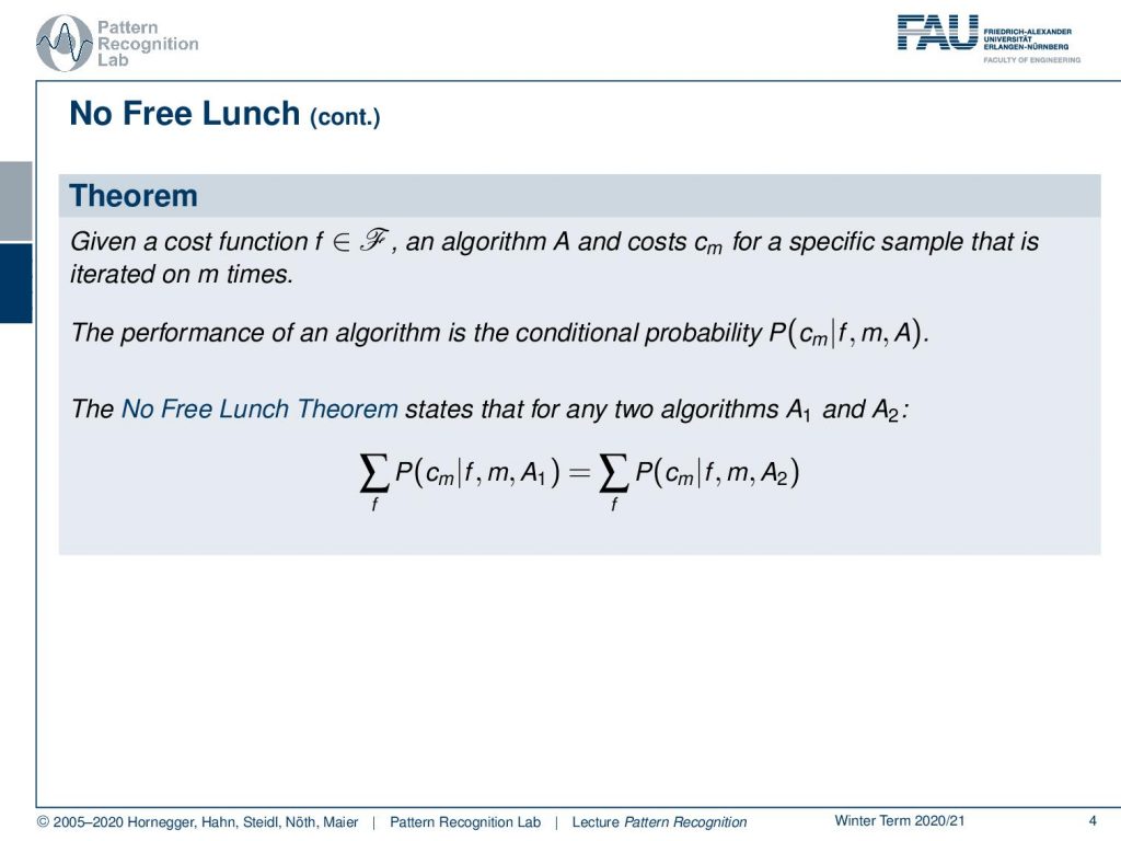
This brings us to the No Free Lunch Theorem and the No Free Lunch Theorem tells us given a cost function f living in the space of cost functions and algorithm A and cost cm for a specific sample and we iterate this m times then the performance of an algorithm is the conditional probability of the cost given the cost function, the iteration, and the algorithm. Now the No Free Lunch Theorem states that for any two algorithms A1 and A2 there is equivalence in terms of the sum over these probabilities over all the possible cost functions. This has a couple of consequences for the classification methods.
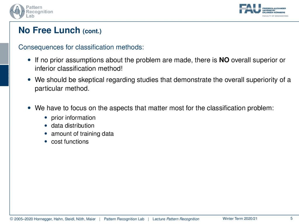
If no prior assumptions about the problem are made, there is no overall superior or inferior classification method. So if you don’t know what the application is and if you don’t know how the cost is actually generated there is no way of picking the best algorithm. So generally we should be skeptical regarding studies to demonstrate the overall superiority of a particular method. If you have a method that shows that for this particular problem this method is suited better then this is probably something that you can believe. If there is a paper that says for all of the problems this algorithm is better than the other algorithm it would be a contradiction to the No Free Lunch Theorem. So we have to focus on the aspects that matter most for the classification problem. There is prior information that is very relevant to improve your classification. The data distribution so you really have to know how your data is distributed how your data behaves. Then, of course, the amount of training data is very relevant for the performance of the classifier and of course the cost function the purpose of how you’re actually designing the classifier.
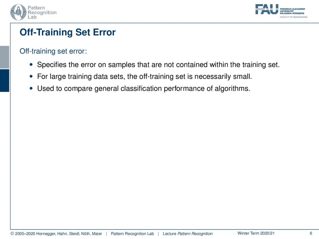
If you consider the off training set error, we are able to essentially measure the performance outside the data that we’ve seen during training. So this is very relevant to measure the performance towards an unseen data sample. So here we need to compute the error on samples that have not been contained in the training set. For large training sets the off training error should be small. So you use it to compare a general classification performance of the algorithms for a particular problem.
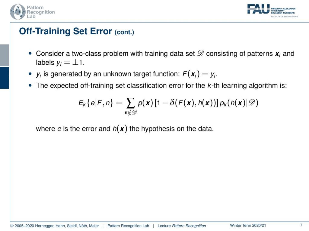
Now if you consider a two-class problem with training dataset D consisting of patterns xi and labels yi then yi is generated by an unknown target function f(xi). and this returns yi. The expected off training set classification error for the cave learning algorithm can then be found as the expected value k of the error given f and n and we compute this as the sum of all the observations of x. This is the probability of x times 1 minus δ(F(x),h(x)), where δ is essentially the hypothesis on the data and then pk(h(x)) given D. So E here essentially is the error that is caused by the hypothesis.
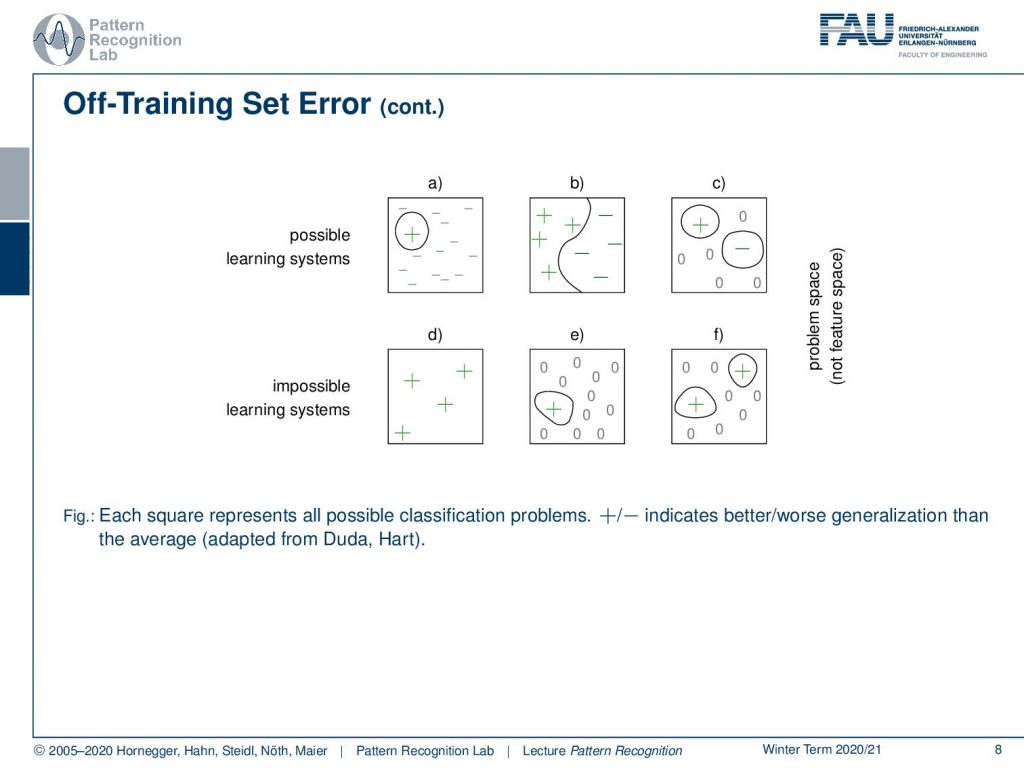
So there are different ways of separating learning systems and you can essentially separate them into possible and impossible learning systems. So possible ones are you have one positive example and many negative ones you have many positive and many negative ones or you could even have positive and negative examples and also outliers rejection classes that are indicated with zeros here. Then there’s also impossible learning systems where you only have positive samples. Then you can’t make any assumptions about the negative class. You can only do things like the distance to the positive samples. You can also have rejection, but it won’t tell you anything about the negative class and essentially if you’re missing any observation any information about the other class then you cannot train any system on this.
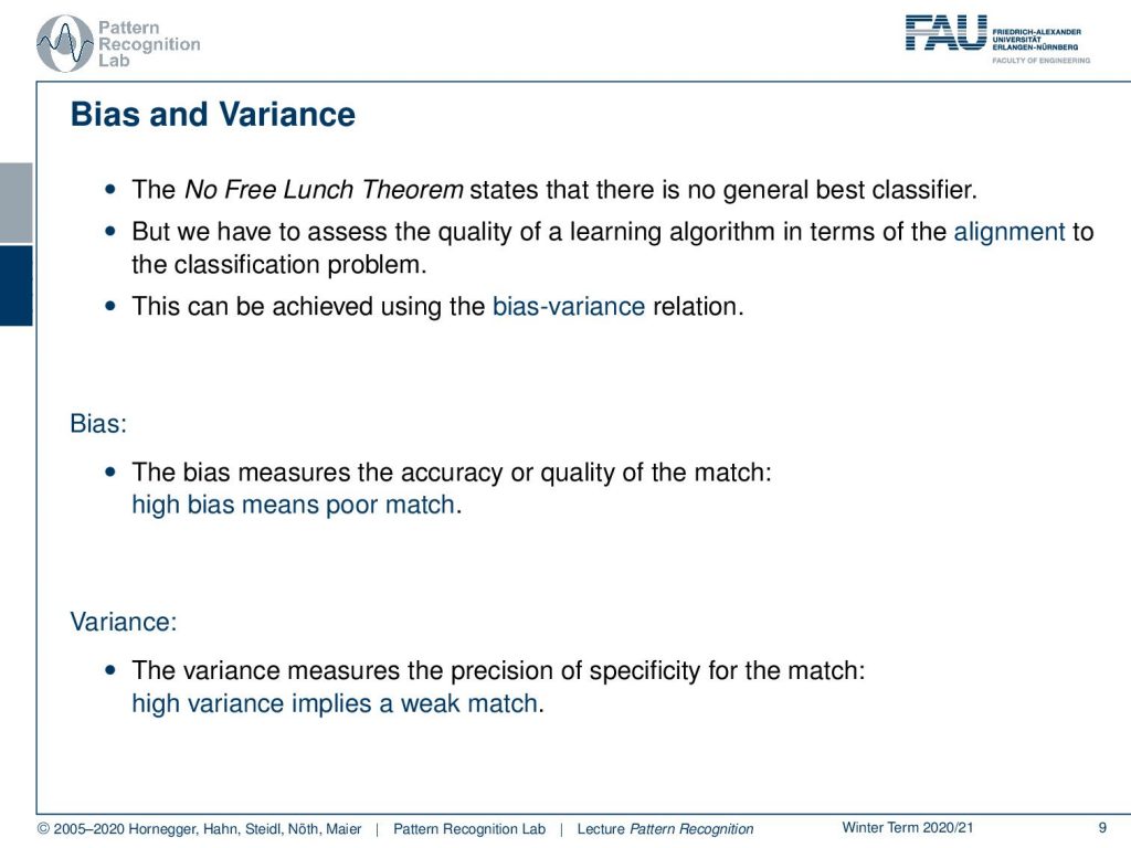
Now the No Free Lunch Theorem tells us that there is no general best classifier. But actually, we have to assess the quality of the learning problem in terms of the alignment to the respective classification problem. This can be done using the bias-variance relation. So the bias measures the accuracy or quality of the match. So high bias means poor match. The variance measures the precision of the specificity for the match. So high variance implies a weak match.
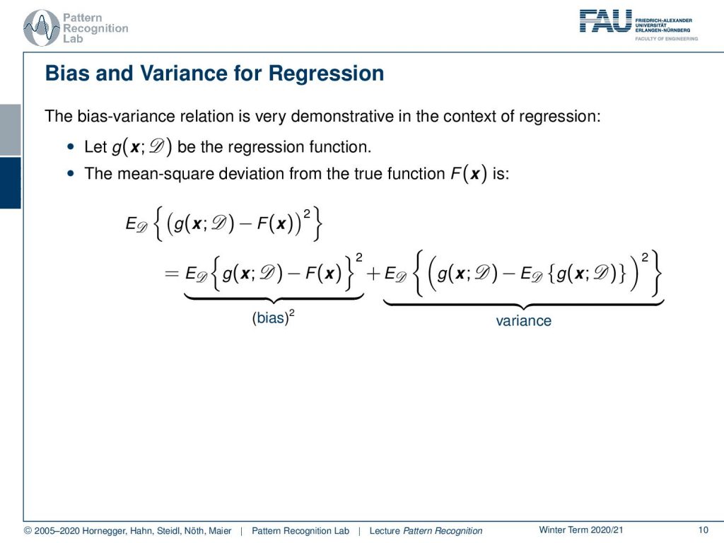
Now the bias-variance relation can be demonstrated very well in the context of regression. So let g(x) be the regression function and then we can compute the mean square deviation from the true function using g. This is going to be the expected value of the difference of the two to the power of two and if you compute this you can essentially determine the bias which is essentially given as the expected value of the difference of the two to the power of two and the variance which is the expected value of the actual function value minus the expected value of the function value. So it is essentially a measure of the variability of the estimation function.
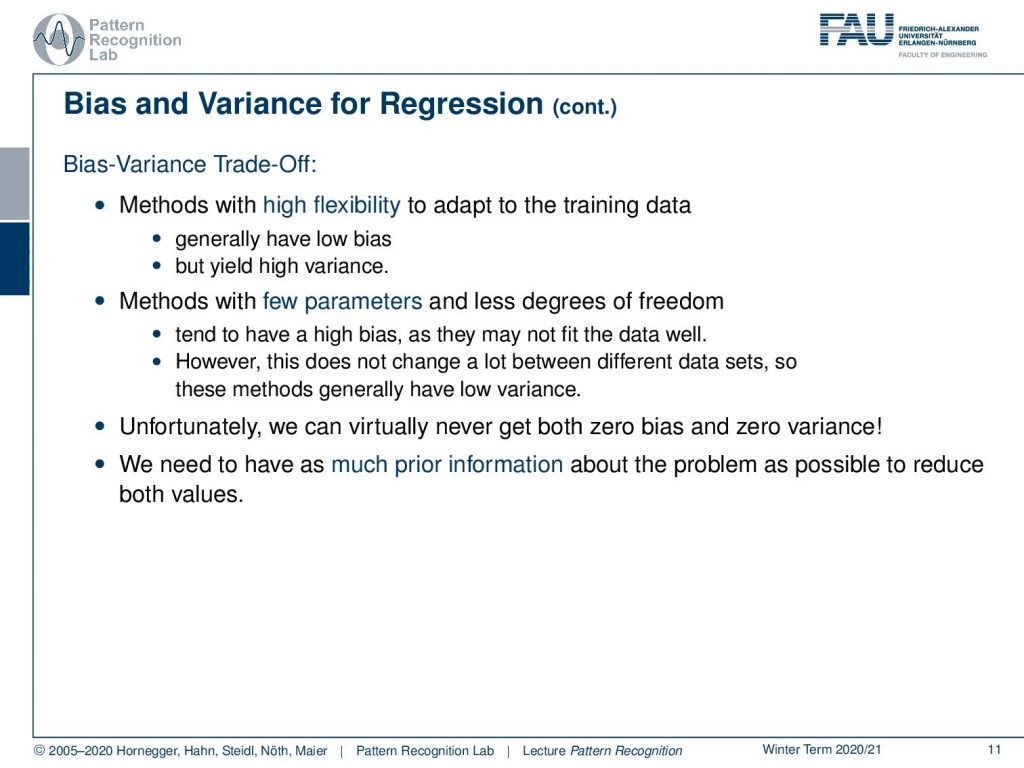
This leads then to the bias-variance trade-off which means that methods with high flexibility try to adapt to the training data. They generally have a very low bias. This also then relates to the model capacity. So we generally have a low bias but we generate a high variance and methods with few parameters and less degrees of freedom. These tend to have a high bias and they may not fit the data as well. However, this does not change a lot between different data sets. So these methods generally have low variance. Unfortunately, we can virtually never get both the bias and the variance to zero. So we need to include as much prior information about the problem as possible to reduce both values.
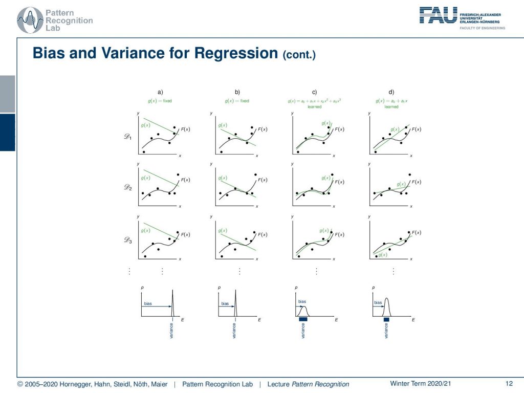
Let’s have a look at some bias and variance examples for regression. So in the first column, you see models that generally have a high bias. Then in the second column, you see models that have a slightly lower bias but again a very limited variance. In the third column, you see a more complex model. So this has a much higher variance and this variance can then be used to reduce the bias. In the last column you see again a model that has a lower variance but this then buys in a certain bias.
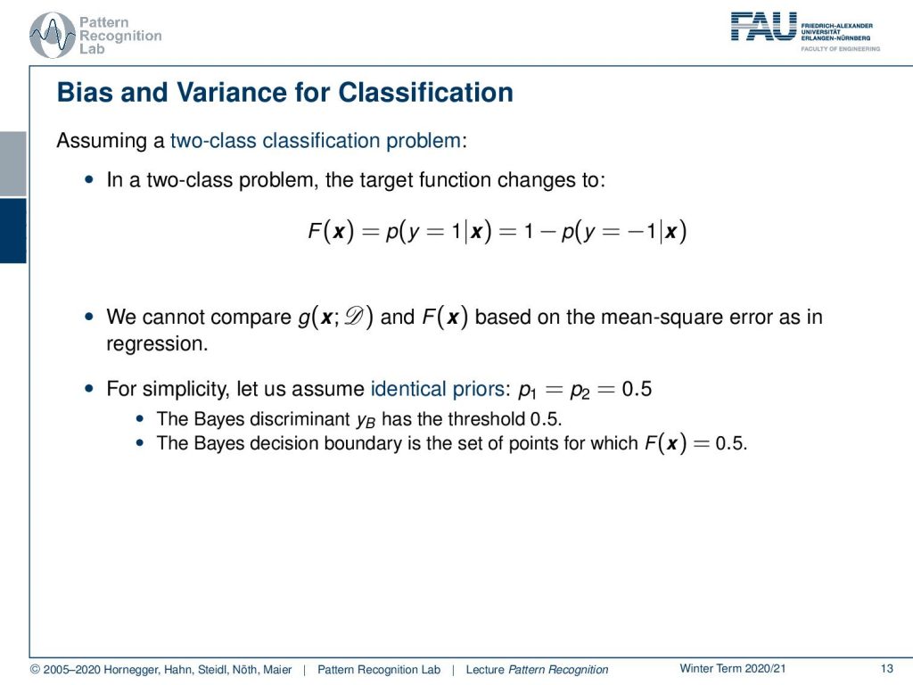
So let’s assume a two-class problem. In a two-class problem, the target function changes to p(y=1|x), and this can be expressed as one minus p(y=-1|x). So here we cannot compare g(x) and F(x) based on the mean square error as in regression. This then means that we have to do a couple of tricks to be able to do that. So we can use for simplicity identical priors p1 equals p2equals to 0.5.
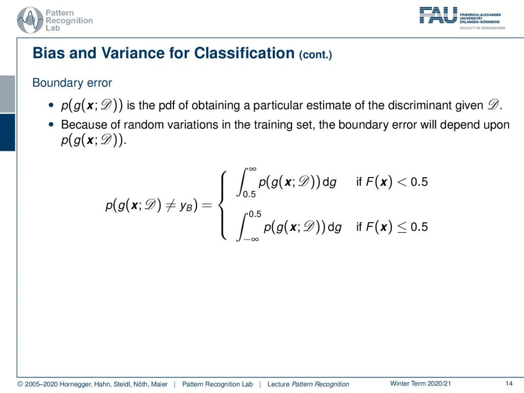
This means that the base discriminant has the threshold of 0.5 and the decision boundary is the set of points for which F(x) equals to 0.5. If we do so then we can essentially get the boundary error that is the probability density function over essentially the models that can be constructed using the data set D. Because of random variations in the training set the boundary error will depend on this probability. So the probability of g being not equal to yB can then be expressed for the two cases for the two classes using those two integral statements.
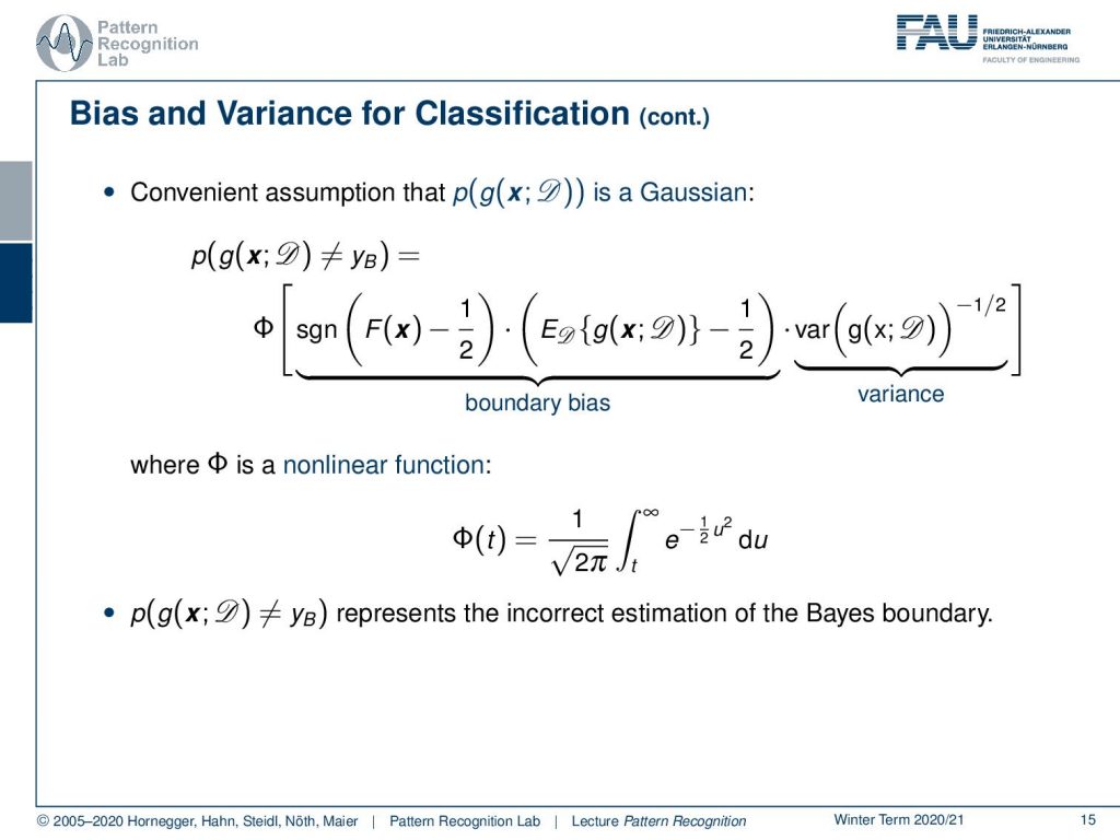
Now if we conveniently assume that our probability density function is a Gaussian, then we can even rewrite this into the following form. Here you then have a non-linear function φ and this is then dependent on the sign of the decision boundary minus 1 over 2 times the expected value of our model minus 1 over 2 times the variance of the model and this to the power of 0.5. So we take the square root of the variance. Now we have this non-linear function φ in here that is given as 1 over the square root of 2π and then the integral from t to infinity over e to the power of minus 1 over 2, u squared and the integral over u.
Now you see that the bias-variance tradeoff for classification is a little bit more complicated. In regression, however, we have this additive relation between bias and variance. For classification, we have multiplicative behavior and non-linearity, and also in classification, the sign of the boundary bias affects the role of the variance in the error. Therefore low variance is generally important for accurate classification. So we can conclude that variant generally dominates bias in classification.
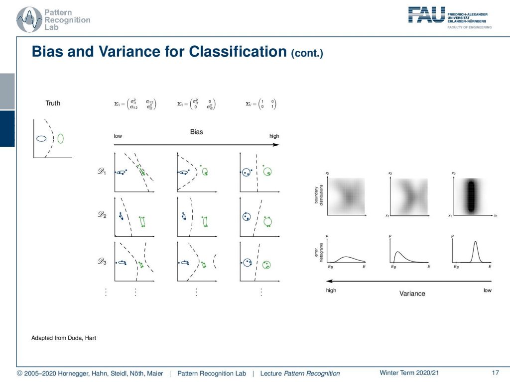
So let’s have a look at some examples here. Again we have models here with low and high bias. You see that this is then directly related to their variance and we can also look at their variances and see that if we have essentially high bias models, then they also can result in lower variance. The models that have a low bias typically have this increase in variance.

So next time we will want to talk a little bit more about the model assessment and in particular, we want to look into ideas on how to generate robust estimates of the performance of the classification system in data sets of limited size. So I hope you like this little video and I’m looking forward to seeing you in the next one. Bye-bye!!
If you liked this post, you can find more essays here, more educational material on Machine Learning here, or have a look at our Deep Learning Lecture. I would also appreciate a follow on YouTube, Twitter, Facebook, or LinkedIn in case you want to be informed about more essays, videos, and research in the future. This article is released under the Creative Commons 4.0 Attribution License and can be reprinted and modified if referenced. If you are interested in generating transcripts from video lectures try AutoBlog
References
- Richard O. Duda, Peter E. Hart, David G. Stork: Pattern Classification, 2nd Edition, John Wiley & Sons, New York, 2000.
- S. Sawyer: Resampling Data: Using a Statistical Jackknife, Washington University, 2005.
- T. Hastie, R. Tibshirani, J. Friedman: The Elements of Statistical Learning, 2nd Edition, Springer, 2009.