Lecture Notes in Pattern Recognition: Episode 18 – Norm-dependent Regression

These are the lecture notes for FAU’s YouTube Lecture “Pattern Recognition“. This is a full transcript of the lecture video & matching slides. We hope, you enjoy this as much as the videos. Of course, this transcript was created with deep learning techniques largely automatically and only minor manual modifications were performed. Try it yourself! If you spot mistakes, please let us know!
Welcome back to Pattern Recognition! Today, we want to look a bit more into how to apply norms in regression problems.
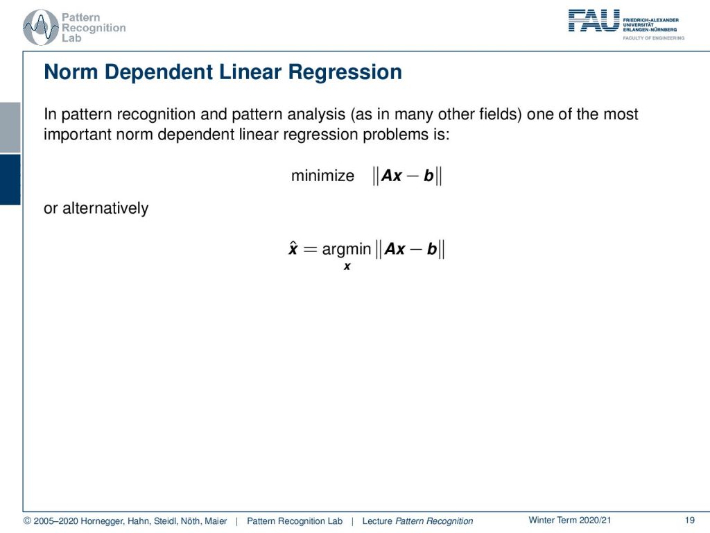
Here you see the norm dependent linear regression. You’ve seen that we essentially now put up the norms that we’ve seen previously in the optimization problem. Here we have some matrix A and some unknown vector x. We subtract this from b and take the norm of this problem. We can write this down as a minimization problem. So, the variable that we’re looking for is determined as the argument of the respective norm problem here.
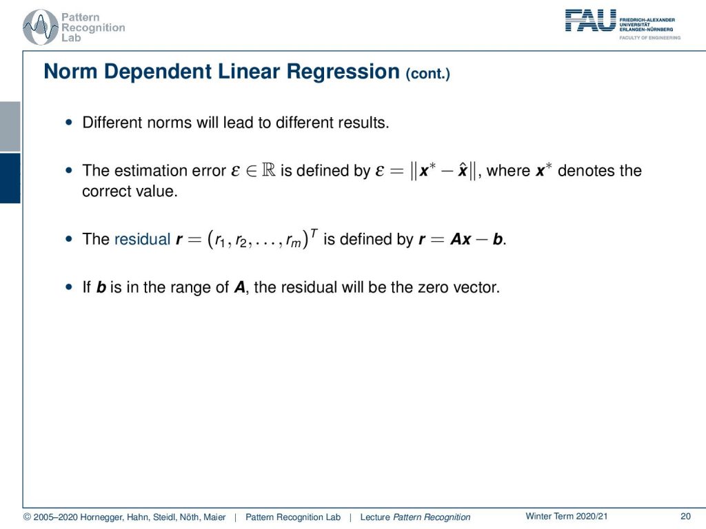
Now different norms will of course lead to different results. And the estimation error ε, which a scalar value, can be defined as the difference between the optimal regression result and the x*, which denotes the correct value. This then gives rise to a residual, so r1, r2, up to rm, where m is the number of observations. They can then be essentially computed as the element-wise deviations from our regression problem. This is essentially nothing else as Ax-b, and the resulting vector gives us the residual terms. If b is in the range of A, the residual will be essentially a zero vector, so it can be completely projected.
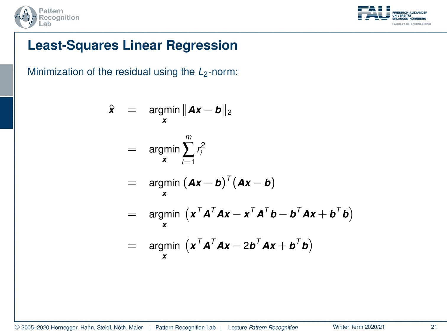
Now, the minimization using the L2-norm is something that we’ve already seen. There, we simply have Ax-b and the L2-norm of that. This can then essentially be rewritten as the minimization over the residuals. You know that the residuals can be expressed as the above norm. So we can write this up also as (Ax-b)T (Ax-b). Now we can do the math. So, I’ve omitted this in the previous video, but now you see the full solution to how to express that. You see that we multiply all the terms with each other. This then gives (xTATAx-xTAT b – bTAx + bTb). Now you see that we can rearrange this a little bit. Two terms are essentially the same if we rearrange them. So, this can be written up as (xTATA x – 2bTAx + bT b).
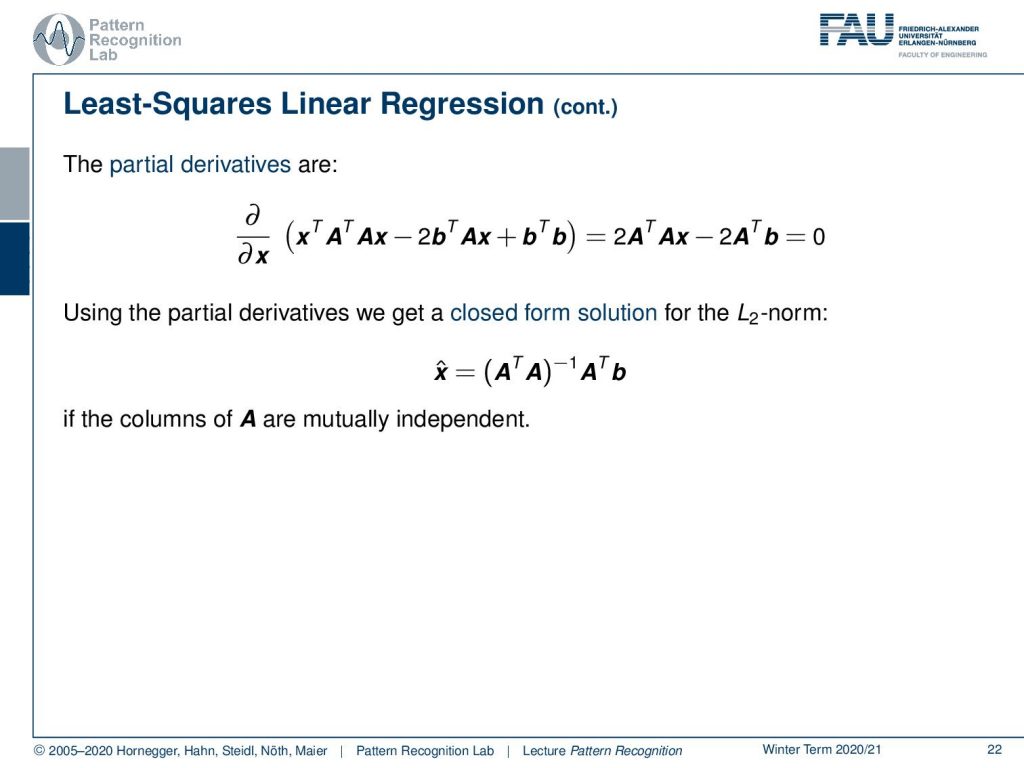
Now, if you want to have the minimization you take the partial derivative of this term with respect to x. And you see now that we can essentially write this up as 2ATAx-2ATb = 0. This then gives the well-known solution of the pseudo inverse for x̂. So, this is (ATA)-1 ATb. This is of course valid if the columns of a are mutually independent. Well, what happens if we do other norms?
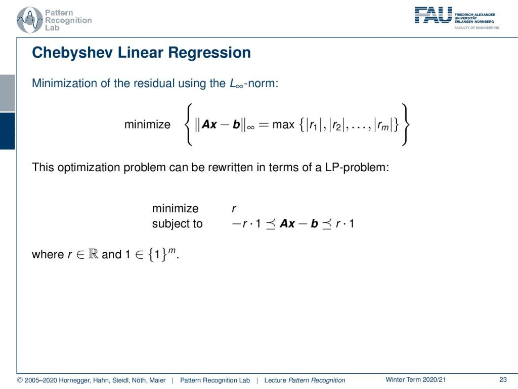
Well, if we do that, then we see we can, for example, use the maximum norm. Here, then the result of the norm would be the maximum over the absolute value of the respective residuals. Then this can also be rewritten into the following optimization problem. We minimize the residuals subject to that the difference of the respective residuals lies between -r times a vector of ones, and the upper bound is r times a vector of ones. So, we are trying to essentially shrink those boundaries as close as possible around our remaining residuals.
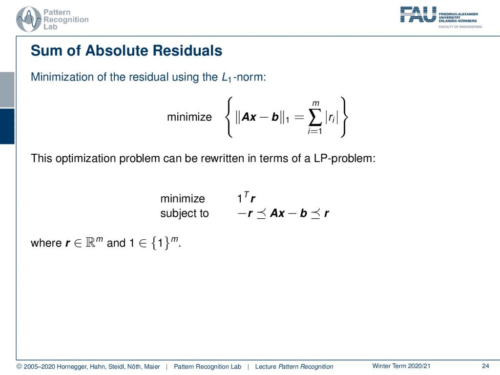
Then we can also look into the minimization of the L1-norm. The L1-norm is the sum over the absolute values over the residuals. This you can rewrite into the minimization problem that we have this vector of 1Tr. Then, this can be used as an upper and then lower bound in the constrained optimization. And again, here our r is a vector in an m-dimensional space and we have this vector of ones only. Let’s look a bit into the application of this!
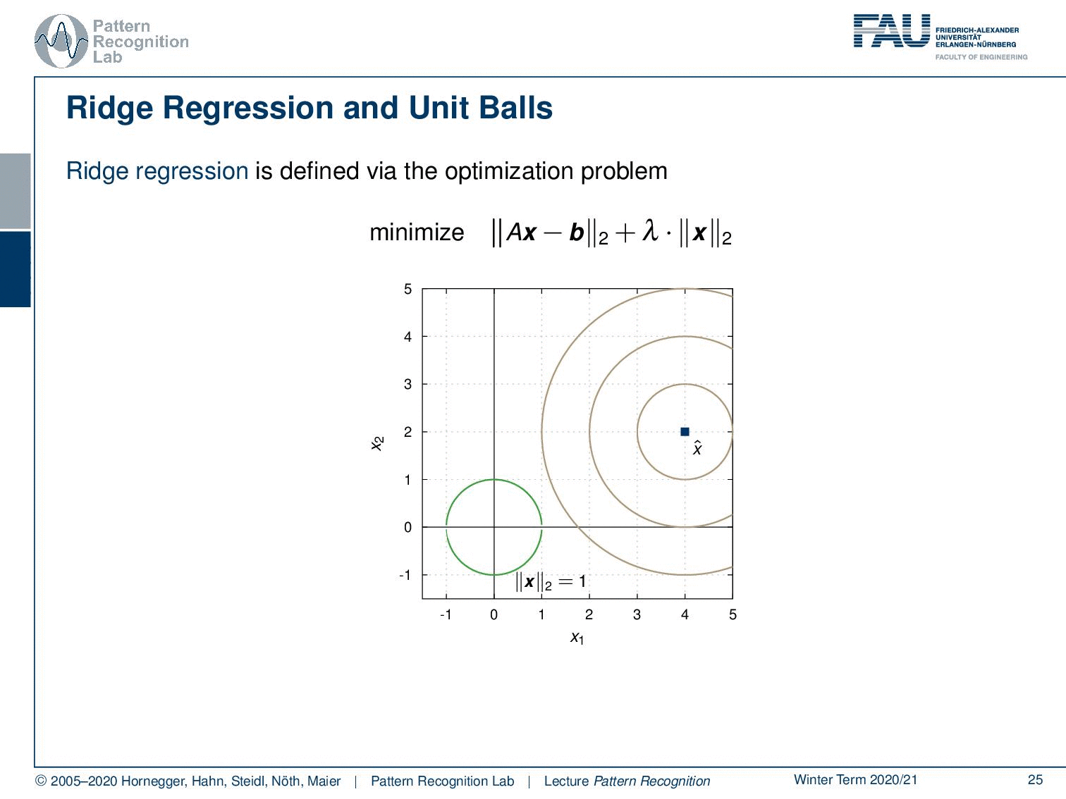
Let’s look into the ridge regression and unit balls. We have here the minimization of Ax-b and the L2-norm times λ the L2-norm of x. Let’s visualize this a little bit. Let’s take the unit ball. The unit ball of x would be exactly this circle here. And now we can look into our actual problem domain. We can gradually increase the circle and then you see if you want the norm exactly to be one you get the hit here. And this will be then the solution for your respective optimization problem. Now, what happens if we take a different norm?
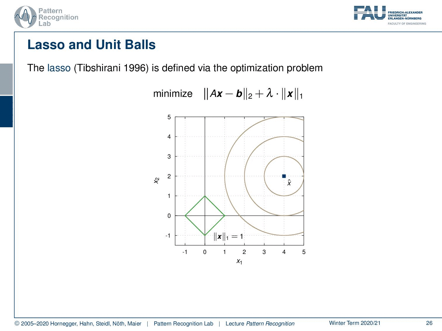
So, let’s take the L1-norm for our x. Again, our original data term is in the L2-norm, but x is regularized with the L1-norm. Then the unit ball looks like this, so we have this diamond shape. And again, we are increasing our data term. Then we see we hit at this position. So, we essentially find the solution that lies on the coordinate axis. And this is also the reason why people like to use the L1-norm. It prefers solutions that lie on the coordinate axis. So, this is why the L1-norm is typically associated with a sparsifying transform. By the way, if you essentially have the L0.5-norm, the effect will be even stronger because you have this peaked shape. And if you have an L0-norm, of course, you will find only sparse solutions. But, of course, this then also results in non-convex optimization problems, which are kind of tricky.
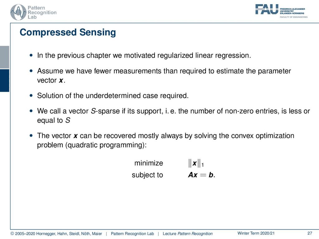
Now let’s look a bit into something that is called compressed sensing. If you work with magnetic resonance imaging or other reconstruction problems, also in CT for example, then the compressed sensing theory is very important. We’re only hinting at this here. If you want to know more about compressed sensing, there are for example classes on magnetic resonance imaging where these concepts are explained in more detail. Here we assume that we have fewer measurements than required to estimate the parameter vector x. So, the solution will be underdetermined and therefore we need regularization. We can call a vector S sparse if its support, meaning the number of non-zero entries, is less or equal to S. Then the compressed sensing tries to find a solution where you essentially minimize the norm of x. So, you try to find a sparse solution for the solution x given to the data term that, for example, Ax = b matches your measured observations. And if you’re able to find these sparse representation transforms, they are typically then also incorporated into the L1-minimization. Then you can reconstruct the original signal from fewer measurements than required to represent, for example, the entire image. And this gives rise to a lot of those savings in x-ray and much more rapid measurements in MRI imaging. So, this is a very important technique that has been used to practice in imaging in many different ways. I really recommend having a look at those specialized lectures. For example, our medical image processing lectures will talk much more about the details of this type of math.
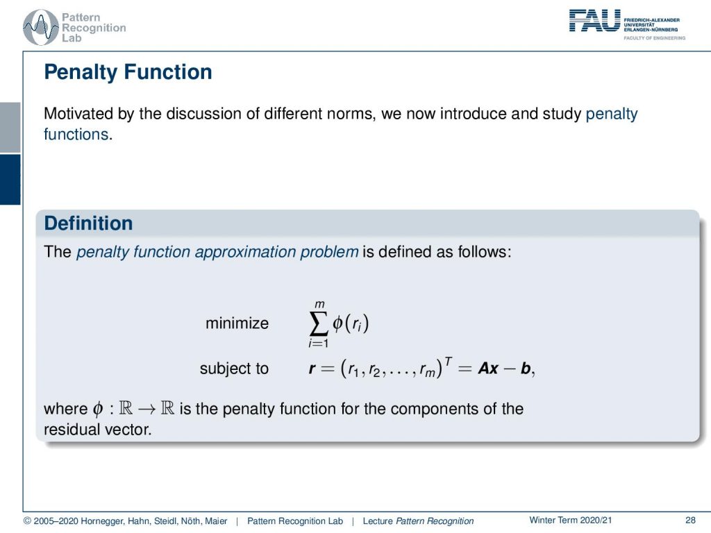
Let’s look a bit into the so-called penalty functions. This is motivated by the discussion of the different norms. We can use that to express certain ways of constraining our regularization. There, you then introduce some function Φ that is applied to the residual. Then you sum up all of the residuals after applying Φ. And then again, you have the constraint that the solutions should follow the data observation, so our Ax-b.
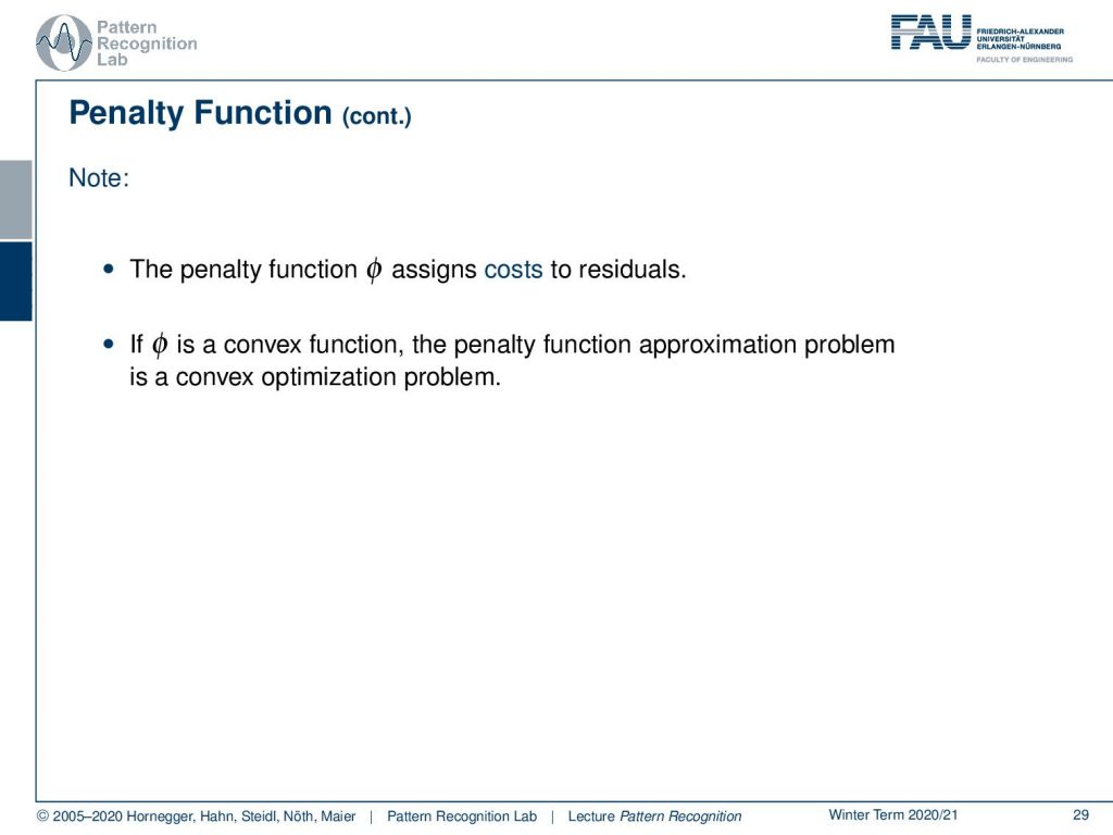
If we do that, then we can find penalty functions very easily. The dependency function plays the role that it assigns a cost to the residuals. And if Φ is a convex function, then the penalty function approximation problem is also a convex optimization problem.
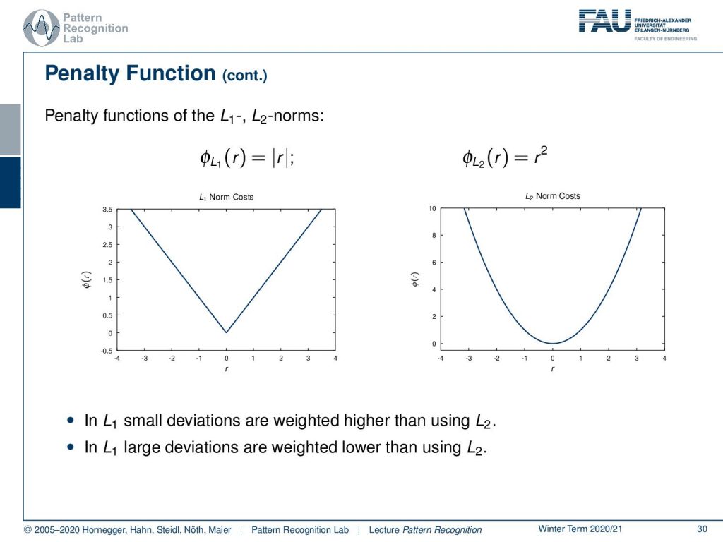
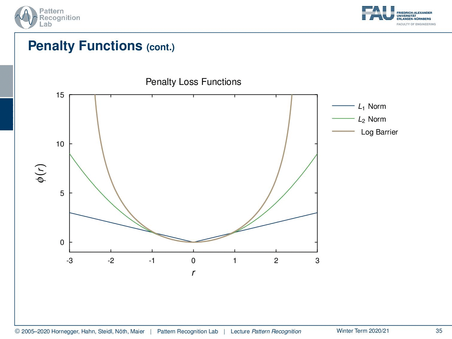
Let’s look into some of those. You can already see that we can now reuse our norms. So, for the L1-norm, it’s simply the absolute value, and for the L2-norm, it’s simply the square. Then, this gives rise to the following penalty functions. Here you can see, for example, that the L2-norm punishes outliers much more rapidly because it’s increasing much more rapidly. Therefore, outliers also have a pretty strong influence on any kind of L2 optimization, while in the case of the L1-norm, the outliers, so things that are far away from zero, are not punished as strongly. So typically, also L1 regularizations are known to be more robust.
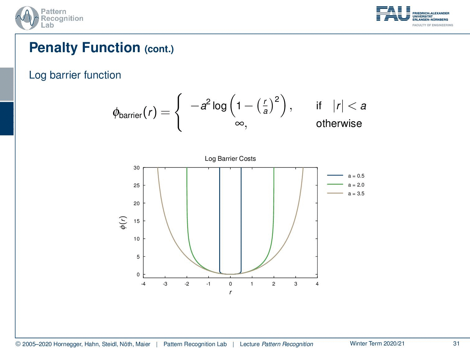
So, let’s look into more penalty functions. A very well-known one is the so-called log barrier function. This is chosen to be essentially constrained around a certain area within the region a. As soon as you leave this area your penalty will be infinite. So, this is then often used to prevent solutions that would essentially go into areas beyond a, and they would have an infinite penalty. Therefore, these solutions are not feasible for your minimization problem. You can vary this a little bit. So, if I increase the area of a, then you see that we also have a solution that is not as strongly regularized.
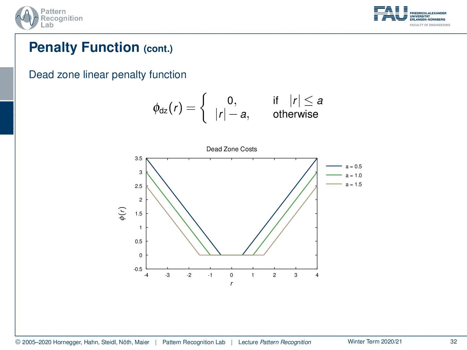
There are also dead zone linear penalty functions. Here you essentially start introducing zones that do not receive any penalty. So, everything in a closed region in the vicinity of zero doesn’t cause any penalty, and only if you move away from there you introduce a penalty. Of course, you can vary this function as well.
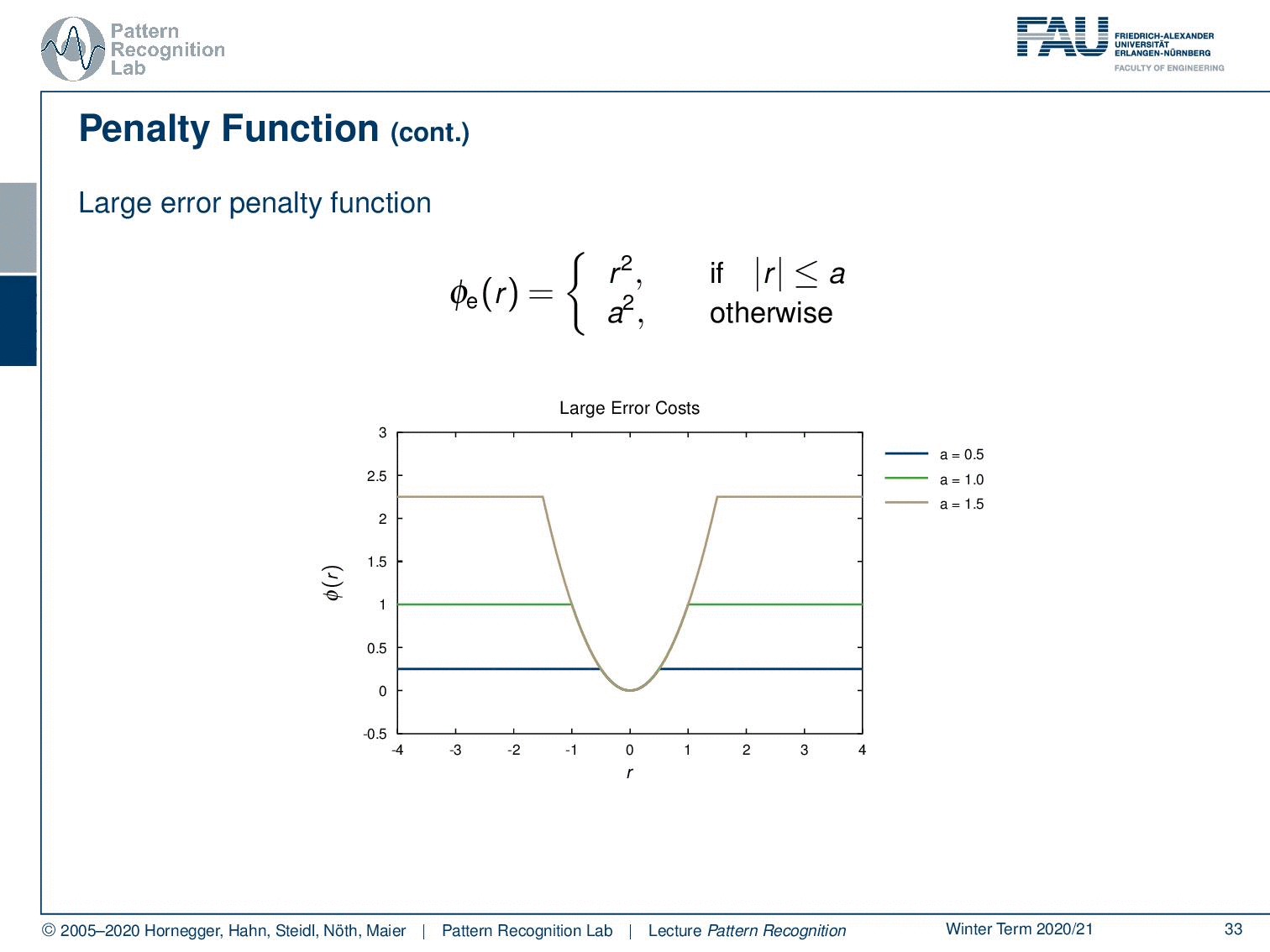
You can have the large error penalty function. Here you essentially define an error that is assigned to large errors so that the error or the penalty is going to be a square. as long as you are below a you simply set it to the square of r, so of the residual. And of course, you can vary this one as well. Here you simply say if I do an error it just counts as an error, but I don’t care how strong the error is.
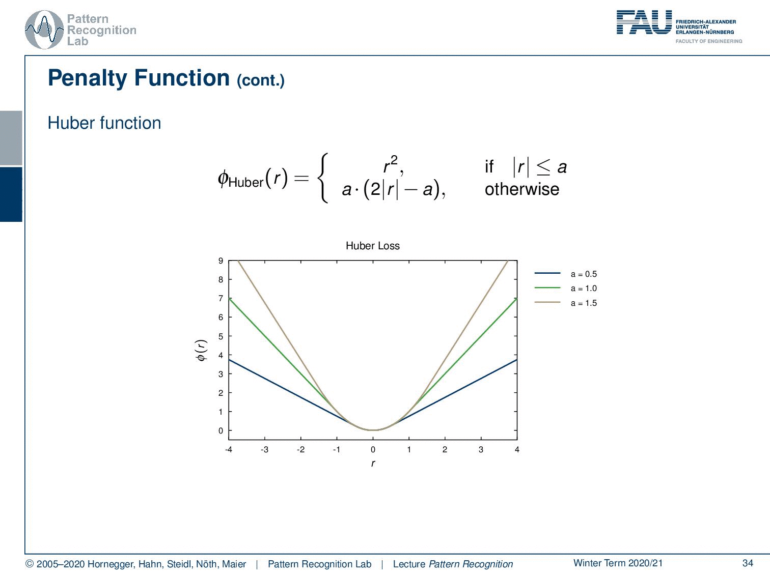
What else? there is the so-called Huber function. Now the Huber function is a differentiable approximation of the L1-norm. Within the area close to zero, so if the absolute value of the residual is below a, we essentially take r2. So, in this part, we have a quadratic behavior. And as soon as we leave a, we just do a linear extrapolation with a linear slope that is continuous in the gradient. So essentially, we can also compute derivatives on this one very nicely. We don’t have to deal with the kinks that are for example introduced in the L1-norms. So, we also have different variants of the Huber norm, and you see that it behaves linearly outside of the area close to zero.
Then let’s compare them a little bit. This is the L1-norm, this has a kink. So, if you want to go towards optimization of this one, you have to deal with sub-gradients, and you also probably then want to use shrinkage kind of optimization programs. If you’re interested in sub-gradients and how to deal with functions that have a kink in optimization effectively, I can really recommend going to our lecture Deep Learning. There we have plenty of functions with kink and it can also be solved. But if you prefer to remain in the domain of a simple gradient, then you can work with simple L2-norms. We’ve also seen the log barrier norm that is shown here, where we essentially then have an infinite penalty as soon as we leave the target domain. Then we also have these dead zone penalty functions, again we have a kink here. Also, optimization is a little bit trickier. But again, sub-gradient saves the day. And then there’s the large error function. Again, we have the kink, and this is then also a non-convex function. So, we kind of will have to deal with non-convex optimization problems here as well. This is the Huber loss. The Huber loss is very popular, or was very popular, as an approximation of the L1-norm with a continuous derivative. So, this has been used widely in the literature. Today you don’t find it as often because most of the time people are simply using the respective L1-norm and shrinkage methods to solve the problem.
So, what are the lessons that we learned here? We have considered vector and matrix norms in more detail. We have seen that there are important norms. The ones that we encounter quite frequently are the L1-norm, L2-norm, L∞, and the LP-norm. We also looked into the respective unit balls. We’ve seen that we can use them for linear regression as well and that they range from closed-form solutions to LP-problems to solve them. Also, the regularized linear regression can range from close form solutions through QP-problem and combinatorial optimization problems in particular if you go to the non-convex cases. So, depending on the objective function that you are setting up here, you have to know the properties, and then you also have to know which algorithm to apply to solve it effectively. And there you need to know the basics of constraint and unconstrained optimization as well as convex optimization. If you want to know more about convex optimization, I really recommend having a look at the lecture of Stephen Boyd at Stanford. It’s a very nice lecture that gives you all the different ideas on how to deal with convex optimization problems.

Next time in Pattern Recognition we want to start looking into a new class of optimization problems and in particular, things that are used in neural networks. Also, we will start with the basic perceptron, and then go ahead and derive them up to neural networks.
I also have some further readings for you. I can tell you that the book by Golub is very good, “Matrix Computations”. Then again, the “Numerical Linear Algebra”. And, as I already mentioned, the book by Boyd and Vandenberghe, “Convex optimization”. There’s also a very good video lecture online available, so I recommend having a look at that.
And of course, we do have some further readings. There is a very nice toolbox on compressed sensing, which is a very hot topic.
And I do have comprehensive questions for you that will help you with the preparation for the exam.
Thank you very much for listening and I’m looking forward to meeting you in the next video! Bye-bye.
If you liked this post, you can find more essays here, more educational material on Machine Learning here, or have a look at our Deep Learning Lecture. I would also appreciate a follow on YouTube, Twitter, Facebook, or LinkedIn in case you want to be informed about more essays, videos, and research in the future. This article is released under the Creative Commons 4.0 Attribution License and can be reprinted and modified if referenced. If you are interested in generating transcripts from video lectures try AutoBlog.
References:
G. Golub, C. F. Van Loan: Matrix Computations, 3rd Edition, The Johns Hopkins University Press, Baltimore, 1996.
Lloyd N. Trefethen, David Bau III: Numerical Linear Algebra, SIAM, Philadelphia, 1997.
S. Boyd, L. Vandenberghe: Convex Optimization, Cambridge University Press, 2004. http://www.stanford.edu/~boyd/cvxbook
http://www.dsp.ece.rice.edu/cs
http://people.ee.duke.eu/%7Elcarin/compressive-sensing-workshop.html